Six Elements, One Comparison — Tensorgami archive

This booklet starts with addition modulo six and follows one example through the comparison argument behind Jordan–Hölder. The calculation uses subgroups and cosets. Read §§1–8 as the main route. Section 9 is an optional spectral calculation, §§10–11 contain exercises and answers, and §12 is a guide to the higher chapters. References marked main § lead to the full exposition.

1 · Two chains through the same six elements

Write $C_d=\Z/d\Z$ . Let

G=\Z/6\Z,\qquad A=\{0,3\},\qquad B=\{0,2,4\}.

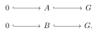
All arithmetic in $G$ is modulo six. We write $0$ for the subgroup $\{0\}$ , which has one element. Consider

Two rows of subgroup inclusions: zero to A to G, and zero to B to G. Here G is the additive group Z/6Z, A is {0, 3}, B is {0, 2, 4}, and zero denotes the trivial subgroup.

Every subgroup here is normal because $G$ is abelian. The factors are

	$\text{first step}$	$\text{second step}$
$A\text{-chain}$	$A/0\cong C_2$	$G/A\cong C_3$
$B\text{-chain}$	$B/0\cong C_3$	$G/B\cong C_2 .$

These identifications are explicit: send $3\in A$ to $1\in C_2$ , send $2\in B$ to $1\in C_3$ , and use reduction modulo three and modulo two for the two quotients of $G$ . Every nonzero element of $C_2$ or $C_3$ generates its group, so these factors are simple.

We can already see the same factors in a different order. Our task is to construct the comparison that makes this inevitable, without assuming that the number of factors is invariant.

Two elementary observations will do much of the work:

A\cap B=0,\qquad A+B=G.

The first follows from the displayed lists. For the second, adding $0$ to the elements of $B$ gives $0,2,4$ , and adding $3$ gives $3,5,1$ . Thus every element has an expression $a+b$ . This expression is unique: if $a+b=a'+b'$ , then $a-a'=b'-b\in A\cap B=0$ .

Main route: main §3, the general refinement theorem, and main §4.4, the $C_6$ comparison.

2 · An algebraic maneuver is a map

Start with $a=b+c$ . To recover $b$ , translate by $-c$ . The translation $\tau_c(x)=x+c$ is a bijection of the underlying set, with inverse $\tau_{-c}$ , because associativity gives

(x+c)+(-c)=x+(c-c)=x.

Thus subtraction is the application of an inverse map. A translation is usually not a group homomorphism: it need not preserve zero.

Distributivity says something different. The homomorphism $h(x)=2x$ satisfies

h(x+c)=h(x)+h(c),

A commutative square with G at all four corners. The top map is translation tau_c, both downward maps are h, and the bottom map is translation tau_{h(c)}. Thus h composed with tau_c equals tau_{h(c)} composed with h. In this example h(x) = 2x.

The square says $h\circ\tau_c=\tau_{h(c)}\circ h$ : applying $h$ before or after the appropriate translation gives the same result. For a vector space the same statement holds for multiplication by a scalar; for a nonzero scalar that linear map is also invertible.

Now consider the quotient map $q_A:G\to G/A$ , $x\mapsto x+A$ . Its fibers are

\{0,3\},\qquad\{1,4\},\qquad\{2,5\}.

Addition of cosets is well defined: replacing $x,y$ by $x+a,y+a'$ , with $a,a'\in A$ , changes $x+y$ by the element $a+a'$ of $A$ .

Suppose $h:G\to H$ is a group homomorphism constant on these fibers. Then there is a unique homomorphism $\bar h:G/A\to H$ such that

\bar h(x+A)=h(x),

The fiber condition proves independence of the representative; the homomorphism law follows from that of $h$ ; surjectivity of $q_A$ proves uniqueness. This is descent through a quotient.

For a concrete instance, $h(x)=4x$ lands in $B$ and kills $3$ . Consequently

\beta:B\longrightarrow G/A,\quad b\longmapsto b+A, \qquad \gamma:G/A\longrightarrow B,\quad x+A\longmapsto4x

are inverse homomorphisms. Indeed, $4b=b$ for $b\in B$ , and $4x-x=3x\in A$ for every $x\in G$ .

Inversion reverses the translation, distributivity gives the compatibility equation, and constancy on fibers allows the map to descend through the quotient.

Further development: main §1, relations, images and quotients.

3 · Keep the identifications, including where they live

A relation $R$ from $X$ to $Y$ is a set of pairs $(x,y)$ . Write $xRy$ for membership. Its input support consists of the $x$ 's occurring in a pair; its output support consists of the $y$ 's occurring in a pair. A relation may have several outputs or none.

For a subgroup $D\leq G$ , write $\Delta_D=\{(d,d):d\in D\}$ . Encode our four quotient steps by

$\text{relation}$	$\text{rule}$	$\text{support}$	$\text{class of }0$
$r_1$	$x=y\in A$	$A$	$0$
$r_2$	$y-x\in A$	$G$	$A$
$s_1$	$x=y\in B$	$B$	$0$
$s_2$	$y-x\in B$	$G$	$B .$

Thus $r_1=\Delta_A$ records $A\to A/0$ , whereas $r_2$ records $G\to G/A$ : two elements are related exactly when their quotient images agree. Each is an equivalence relation on its support. Viewed on all of $G$ , it is a partial equivalence relation. For instance, $1$ is not related to itself by $r_1$ .

Let $Q(r)$ mean the support modulo this equivalence relation. Then $Q(r_1)=A$ and $Q(r_2)=G/A$ . In groups, a congruence is determined by its identity class. The more general argument retains the whole relation, so it need not assume this group-specific fact.

Our convention is that $SR$ means first $R$ , then $S$ :

x(SR)z\quad\Longleftrightarrow\quad \text{there is }y\text{ with }xRy\text{ and }ySz.

The opposite relation $R^\op$ reverses every pair. Associativity of composition is now a statement about witnesses: both $T(SR)$ and $(TS)R$ relate $x$ to $w$ precisely when there are $y,z$ with $xRy,\ ySz,\ zTw$ . Regrouping changes the parentheses, not the data.

For the group argument we use internal relations: subgroups $R\leq X\times Y$ , not arbitrary subsets. Such a relation has the three-corner property

xRy,\quad x'Ry,\quad x'Ry' \quad\Longrightarrow\quad xRy'.

Indeed, closure under multiplication and inversion gives

(x,y)(x',y)^{-1}(x',y')=(x,y').

The order displayed works even in noncommutative groups. This property is called difunctionality; it is the key relation identity supplied by the Mal'cev framework.

Main §§1–2 develop the same operations using pullbacks, regular images and effective quotients, so that they apply beyond groups.

4 · A comparison with two outputs per input

Before filling a whole comparison table, examine the relation

R=r_2s_1,\qquad bRy\quad\Longleftrightarrow\quad b\in B\ \text{and}\ y-b\in A.

First $s_1$ requires the input to be an element of $B$ and leaves it fixed. Then $r_2$ allows movement by an element of $A$ . Its six pairs are displayed by

$\text{input}$	$\text{possible outputs}$
$0$	$0,\ 3$
$2$	$2,\ 5$
$4$	$4,\ 1 .$

The input support is $B$ ; the output support is all of $G$ . There is no single output in the definition.

There are two kinds of ambiguity to remove. Define

E=R^\op R,\qquad F=RR^\op.

Two inputs are $E$ -related when they share an output. The three rows of the table are disjoint, so $E=\Delta_B$ . Two outputs are $F$ -related when they share an input. Hence $F=r_2$ , with classes $\{0,3\},\{2,5\},\{4,1\}$ .

After quotienting, the two possible outputs in each row become one:

B/E=B\xrightarrow[\cong]{\ \beta\ }G/F=G/A,\qquad b\longmapsto b+A.

We proved the inverse formula $x+A\mapsto4x$ in §2. The relation therefore produces an actual isomorphism, with no choice of representatives in its definition.

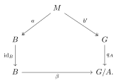
Here is the same construction as a diagram. Let $M=R$ , regarded as a subgroup of $B\times G$ , and take its coordinate projections $a(b,y)=b$ and $b'(b,y)=y$ :

The relation carrier M maps surjectively to B by a and to G by b-prime. B maps down to B by its identity, G maps down to G/A by q_A, and beta maps B to G/A across the bottom. The diagram commutes: beta composed with a equals q_A composed with b-prime. Here a(b,y) = b, b-prime(b,y) = y, and beta(b) = b+A.

Both projections are onto their supports. The equation $\beta a=q_A b'$ says that related elements receive matching quotient images. It characterizes $\beta$ uniquely because $a$ is surjective.

This is the concrete instance of the common-quotient construction in main §2.

5 · Why the construction works beyond six elements

Let $R\leq X\times Y$ be any subgroup relation. Restrict to its input and output supports $X'\leq X$ , $Y'\leq Y$ . Set $E=R^\op R$ and $F=RR^\op$ . They are reflexive on these supports and symmetric by definition.

For transitivity of $E$ , suppose $x,x'$ share output $y$ , and $x',x''$ share output $z$ . The three corners $xRy,\ x'Ry,\ x'Rz$ give $xRz$ , so $x,x''$ share $z$ . Interchanging input and output proves transitivity of $F$ . Thus $E,F$ are equivalence relations on their supports.

They respect the group operations. For example, witnesses $y,v$ for $xEx'$ and $uEu'$ give witness $yv$ for $(xu)E(x'u')$ ; inversion of a witness gives the corresponding inverse relation. The same holds for $F$ . Their classes therefore carry well-defined quotient group structures.

Define

\theta:X'/E\longrightarrow Y'/F,\qquad [x]_E\longmapsto[y]_F \quad\text{whenever }xRy.

An output exists by the definition of support. Different outputs for the same $x$ are $F$ -related. If $xEx'$ , choose a common output $y_0$ ; any outputs for $x$ and $x'$ are each $F$ -related to $y_0$ . Hence the formula is independent of both choices. Reversing $R$ constructs its inverse. Finally, $xRy$ and $uRv$ imply $(xu)R(yv)$ , so $\theta$ is a homomorphism.

This proof is the small mechanism inside the comparison theorem:

\boxed{\text{a compatible relation} \ \longrightarrow\ \text{two ambiguity quotients} \ \longrightarrow\ \text{one canonical isomorphism}.}

The abstract framework packages precisely the operations just used:

Structure	Work it performs
Finite limits	Form pairs satisfying equations and the spaces of witnesses.
Regular images	Form supports and compose relations.
Barr exactness	Make equivalence relations into effective quotients.
Mal'cev property	Supply the three-corner property for internal relations.
Pointedness	Supply a zero object and zero classes for the later series argument.

Pointedness is needed for that formulation of normal series, not for the common-quotient construction itself. Groups and modules provide these structures; the full exposition establishes the categorical relation calculus before using it.

This page proves the group mechanism. The proof for every exact Mal'cev category, with its image and quotient dependencies, is in main §1 and main §2.

6 · Fill all four crossings

Write $A_0=B_0=0,\ A_1=A,\ B_1=B,\ A_2=B_2=G$ . For every pair of quotient steps form

P_{ij}=r_i s_j.

Inputs come from the column side; outputs come from the row side. Because partial equivalence relations are symmetric and idempotent,

P_{ij}^{\op}P_{ij}=s_jr_i s_j,\qquad P_{ij}P_{ij}^{\op}=r_i s_jr_i.

The previous page supplies the canonical map from the input ambiguity quotient to the output ambiguity quotient. Here every cell is explicit:

$(i,j)$	$P_{ij}$	$\text{input quotient}$	$\text{output quotient}$
$(1,1)$	$\{(0,0)\}$	$0/0$	$0/0$
$(1,2)$	$\{(x,3x):x\in G\}$	$G/B$	$A/0$
$(2,1)$	$\{(b,b),(b,b+3):b\in B\}$	$B/0$	$G/A$
$(2,2)$	$G\times G$	$G/G$	$G/G .$

The two nontrivial isomorphisms are

\theta_{12}:G/B\xrightarrow{\sim}A,\quad x+B\longmapsto3x, \qquad \theta_{21}:B\xrightarrow{\sim}G/A,\quad b\longmapsto b+A.

For $P_{12}$ , the intermediate point must lie in $A$ and in the $B$ -coset of the input. It is $0$ for even inputs and $3$ for odd inputs, exactly $3x$ . The formula descends because $3B=0$ . Its inverse is $a\mapsto a+B$ : $3a=a$ on $A$ , and $3x-x=2x\in B$ .

For $P_{22}$ , any input $x$ and output $y$ have an intermediate point $z$ with $z-x\in B$ and $y-z\in A$ , since $A+B=G$ . Thus every pair is related. Both ambiguity quotients are trivial. This cell has support $G$ , whereas the first cell has support $0$ .

Arrange the resulting factors by their original steps:

	$B/0$	$G/B$
$A/0$	$0$	$C_2$
$G/A$	$C_3$	$0 .$

The $C_2$ cell compares the first $A$ -step to the second $B$ -step; the $C_3$ cell compares the other two steps.

There is still a logical obligation: the cells must assemble into genuine refinements of the original chains. A table of isomorphic quotients by itself would not establish a refinement theorem.

7 · How cells become genuine refinements

In this abelian example the refined subgroups have familiar formulas:

U_{ij}=A_{i-1}+(A_i\cap B_j),\qquad V_{ji}=B_{j-1}+(B_j\cap A_i).

For each fixed row or column, let the other index run from $0$ to $2$ :

	$j=0$	$j=1$	$j=2$
$U_{1j}$	$0$	$0$	$A$
$U_{2j}$	$A$	$G$	$G$

	$i=0$	$i=1$	$i=2$
$V_{1i}$	$0$	$0$	$B$
$V_{2i}$	$B$	$G$	$G .$

The output quotient in cell $(i,j)$ is $U_{ij}/U_{i,j-1}$ ; the input quotient is $V_{ji}/V_{j,i-1}$ . Checking these against the previous table gives the two refinements

0\subseteq0\subseteq A\subseteq G\subseteq G,\qquad 0\subseteq0\subseteq B\subseteq G\subseteq G.

Repeated terms contribute trivial factors and can later be deleted.

Why these intermediate subgroups? Let $q_i:A_i\to A_i/A_{i-1}$ . Take the image of $A_i\cap B_j$ downstairs and pull it back:

q_i^{-1}\bigl(q_i(A_i\cap B_j)\bigr) =A_{i-1}+(A_i\cap B_j)=U_{ij}.

Indeed $q_i(x)=q_i(c)$ says exactly $x-c\in A_{i-1}$ . The pullback includes every representative of each chosen coset. For example, in the second row the downstairs chain $0\subseteq G/A\subseteq G/A$ pulls back to $A\subseteq G\subseteq G$ .

This explains saturation: a relation downstairs must lift to all representatives upstairs. For our $R\subseteq B\times G$ , changing an output by $3$ keeps the pair in $R$ ; in formulas $r_2R=R$ . Compare the smaller subgroup relation

T=\{(b,b):b\in B\}\subseteq B\times G.

Under $\id_B\times q_A$ , both $T$ and $R$ have image $\{(b,b+A):b\in B\}$ . But the inverse image of this graph is $R$ , not $T$ : it includes $(b,b+3)$ too. Thus $r_2T=R\ne T$ . Taking an image and pulling it back need not recover unsaturated data.

In the general relation proof, the row objects have the form $t=r_i s_jr_i$ , and

r_i t r_i=t

follows from $r_i^2=r_i$ . Saturation gives descent and pullback; the boundary identities then make adjacent cells meet. The full proof checks both requirements. Our two tables exhibit their result explicitly.

For the categorical descent and boundary checks, see main §2 and main §3.

8 · Why simplicity turns comparison into a matching

Read the rectangle rowwise to get $0,C_2,C_3,0$ ; read it columnwise to get $0,C_3,C_2,0$ . Delete the trivial factors. The matching is given by actual maps:

A\xrightarrow{\sim}G/B,\quad a\longmapsto a+B, \qquad B\xrightarrow{\sim}G/A,\quad b\longmapsto b+A.

No equality of lengths was needed to build these maps.

Here is the general final step for groups. A finite normal series in a nontrivial simple group $S$ has exactly one nontrivial factor. Look at the first term equal to $S$ . Its preceding term is a proper normal subgroup of $S$ , hence is trivial. Every earlier term is therefore trivial, and every later term is $S$ . Notice that this argument needs only normality in the next term.

The general refinement theorem, proved in main §3, constructs a rectangle of paired factors for two finite normal series. If the original series are composition series, each row is a refinement of a simple quotient, so exactly one nontrivial cell survives in that row. The same holds in each column. Those surviving cells give a bijection between the original factors, with an isomorphism for each matched pair. Equality of the numbers of factors is a consequence of this bijection.

This booklet has computed that construction for $C_6$ and proved its common-quotient mechanism for groups. The main exposition proves the general categorical refinement theorem.

Dimension now follows. For a finite basis $v_1,\ldots,v_n$ of a vector space $V$ over $k$ , put $F_i=\operatorname{span}(v_1,\ldots,v_i)$ . The map

k\longrightarrow F_i/F_{i-1},\qquad a\longmapsto av_i+F_{i-1}

is onto by the definition of span and injective by linear independence. The $k$ -module $k$ is simple: a submodule containing a nonzero $a$ contains $a^{-1}a=1$ , hence every scalar. A second finite basis therefore gives another composition series, and Jordan–Hölder gives the same number of steps. For $V=0$ , every basis is empty, directly by independence.

What this example does not test. $C_6$ is abelian, and the map $A\times B\to G$ , $(a,b)\mapsto a+b$ , is an isomorphism by §1. Thus all our subgroups are ambient-normal and this extension splits. Exercise 6 tests adjacent normality in $A_4$ . Exercise 7 shows that the same simple factors can assemble into different groups.

9 · Optional: the same comparison on successive pages

In the module setting, the two filtrations can instead be compared by the spectral calculation developed in main §7. Here $G$ is a $\Z$ -module, and we use the two-term map $f:X=G\xrightarrow{\id}Y=G$ . Extend $A_i,B_i$ by zero below $0$ and by $G$ above $2$ , and set

F_pX=A_{p-2},\qquad F_pY=B_p.

The shift makes $f$ filtration-preserving. On the initial associated graded page, the only nonzero terms are

$\text{filtration column}$	$1$	$2$	$3$	$4$
$X$	$0$	$0$	$A$	$G/A$
$Y$	$B$	$G/B$	$0$	$0 .$

The differential $d_r$ goes from source column $p$ to target column $p-r$ . There is no same-column map, so $d_0=0$ .

Page 1. The only nonzero differential is

d_{1,3}:A\longrightarrow G/B,\qquad a\longmapsto a+B.

It is the $C_2$ comparison already proved to be an isomorphism. Taking its kernel and cokernel removes both of these entries.

Page 2. The remaining source is $G/A$ in column $4$ , and the remaining target is $B$ in column $1$ . A page-2 differential moves two columns, so $d_2=0$ . One zero differential does not imply stabilization.

Page 3. The representative subgroup for the surviving source is now $B$ : to land three filtration steps lower, an element of $G$ must lie in $B$ . Its identification with the preceding source term is precisely

B\xrightarrow{\sim}G/A,\qquad b\longmapsto b+A.

On these representatives $f$ is the identity $B\to B$ , so $d_{3,4}$ is an isomorphism. If we keep the old $G/A$ coordinate, the same map is $x+A\mapsto4x$ . These are two coordinate descriptions of one differential, not two different maps. Page 4 is zero.

The calculation pairs the $C_2$ 's first and the $C_3$ 's later. It uses the same quotient maps as the rectangle; their page locations depend on the chosen filtrations and shift. The filtration machinery and its convergence are proved in the main exposition, not assumed from Jordan–Hölder. Here we have computed the pages explicitly.

Read this after the concrete rectangle. It is an abelian $\Z$ -module calculation; it does not assert that ordinary abelian spectral sequences apply directly to arbitrary groups.

10 · Seven short exercises

The first five exercises stay with $G=\Z/6\Z$ , $A=\{0,3\}$ , $B=\{0,2,4\}$ . They test the maps, not just the final factor list. Worked answers follow on the next two pages.

Direction and witnesses. For $R=r_2s_1$ , give an intermediate witness showing $2R5$ . Does $5R2$ ? Describe $R^\op=s_1r_2$ . Explain why associativity of relation composition does not allow us to interchange $r_2$ and $s_1$ .
The two ambiguities. Compute $R^\op R$ and $RR^\op$ , including their supports. Why is the first not an equivalence relation on all of $G$ ? Write the induced quotient isomorphism and its inverse.
Three corners. Let $T\leq X\times Y$ be a subgroup, with $X,Y$ possibly noncommutative. Verify the ordered product that completes $(x,y),(x',y),(x',y')$ to $(x,y')$ . For the congruence modulo $B$ , apply it to $(0,2),(4,2),(4,4)$ . Give an arbitrary subset of $C_2\times C_2$ for which the three-corner property fails.
What saturation repairs. Let $T=\{(b,b):b\in B\}\subseteq B\times G$ , and let $p=\id_B\times q_A$ . Show $p(T)=p(R)$ , but $p^{-1}(p(T))=R\ne T$ . Compute $r_2T$ and $r_2R$ . Which relation includes every representative of each output coset?
Reconstruct the rectangle. Without looking at §6, compute all four output quotients and all four input quotients. Recover the two refined chains. Verify that $x+B\mapsto3x$ is inverse to $a\mapsto a+B$ . Explain the different supports of the two trivial cells.
Normal in the next term. Let $A_4$ be the group of even permutations of four symbols, composed from right to left. Inside $A_4$ , let
$H=\{1,(12)(34)\},\qquad V_4=\{1,(12)(34),(13)(24),(14)(23)\}.$
Show that $1<H<V_4<A_4$ is a composition series, but $H$ is not normal in $A_4$ . For the last assertion, conjugate $(12)(34)$ by $(123)$ . Why would a proof considering only ambient-normal subgroups miss this series?
What the factors forget. Give composition series for $C_4$ and $C_2\times C_2$ with the same simple factors. Prove the groups are not isomorphic. Then count the homomorphisms $C_2\to C_4$ and $C_2\to C_2\times C_2$ . What information does this small probe detect that the factor list does not?

Exercises 1–5 check the comparison mechanism. Exercises 6–7 expose two features deliberately invisible in the easy $C_6$ example: non-ambient normality and different ways to assemble the same factors.

11 · Worked answers

1. Direction and witnesses. The intermediate point is $2$ : $2s_12$ and $2r_25$ , since $5-2=3\in A$ . But $5$ is outside the input support $B$ , so $5R2$ is false. The opposite relation has pairs

R^\op=\{(b,b),(b+3,b):b\in B\}.

It has input support $G$ and output support $B$ . First move by $A$ , then require the endpoint to lie in $B$ . Associativity permits regrouping three successive operations; it does not reverse their order. Here $r_2s_1\ne s_1r_2$ , as the supports already show.

2. The two ambiguities. Distinct rows in the relation table have disjoint outputs, so

R^\op R=\Delta_B.

It is reflexive on $B$ , but not on $G$ : for example $(1,1)$ is missing. The other composite is

RR^\op= \{0,3\}^2\ \cup\ \{2,5\}^2\ \cup\ \{4,1\}^2=r_2.

Its support is $G$ , and its three classes are the $A$ -cosets. The quotient map is $B\to G/A,\ b\mapsto b+A$ . Its inverse $x+A\mapsto4x$ is well defined because $4A=0$ . The two identities $4b=b$ on $B$ and $4x-x\in A$ verify both composites directly.

3. Three corners. In the direct product group,

\begin{split} (x,y)(x',y)^{-1}(x',y') &=\bigl(xx'^{-1}x',\,yy^{-1}y'\bigr)\\ &=(x,y'). \end{split}

The subgroup contains this product. Nothing is commuted, so the argument works for arbitrary groups. In the additive $C_6$ example the same operation reads

(0,2)-(4,2)+(4,4)=(0,4),

which indeed belongs to the congruence modulo $B$ .

The subset $\{(0,0),(1,0),(1,1)\}\subseteq C_2\times C_2$ contains three corners but omits $(0,1)$ . It is not a subgroup. Merely having a subset of a product supplies no three-corner property.

4. What saturation repairs. Both images are the graph

L=\{(0,A),(2,2+A),(4,4+A)\}\subseteq B\times G/A.

A pair $(b,y)$ lies in $p^{-1}(L)$ exactly when $y+A=b+A$ , or $y-b\in A$ . This is precisely $R$ . Therefore $r_2T=R$ and $r_2R=R$ . Only $R$ includes all representatives of each output coset; $T$ includes just one.

5. Reconstruct the rectangle. The output and input quotient tables, respectively, are

\begin{pmatrix}0/0&A/0\\G/A&G/G\end{pmatrix}, \qquad \begin{pmatrix}0/0&G/B\\B/0&G/G\end{pmatrix}.

Their row and column chains are

0\subseteq0\subseteq A\subseteq G\subseteq G,\qquad 0\subseteq0\subseteq B\subseteq G\subseteq G.

The formula $x+B\mapsto3x$ is well defined since $3B=0$ . For $a\in A$ , $3a=a$ ; for $x\in G$ , $3x-x=2x\in B$ . These prove both inverse identities. The first trivial cell has support $\{0\}$ , and the last has support $G$ . Each quotient has one element, although their supports and relations differ.

6. Normal in the next term. $V_4$ is abelian, so $H\nml V_4$ . Conjugation by an element of $A_4$ permutes the three double transpositions, so $V_4\nml A_4$ . The successive factors have orders $2,2,3$ , and every group of prime order is cyclic and simple. These steps give a composition series. However,

(123)(12)(34)(123)^{-1}=(23)(14)\notin H.

Thus $H$ is not normal in $A_4$ . The theorem concerns subnormal series, where each term is normal in the next; it cannot be reduced to chains in the lattice of subgroups normal in the whole ambient group.

7. What the factors forget. Use

0<\{0,2\}<\Z/4\Z,\qquad 0<C_2\times0<C_2\times C_2.

Both factor lists are $C_2,C_2$ . The first group has an element of order four, while the second does not, so they are not isomorphic. A homomorphism out of $C_2$ is determined by the image of its generator, which must be killed by two. There are two possibilities in $C_4$ and four in $C_2\times C_2$ . The probe detects their different two-torsion subgroups. The simple factors alone do not recover how those factors are assembled.

12 · A guide to the higher chapters

The comparison theorem is already complete before the higher chapters. Those chapters pursue a new question: what additional structure is retained by richer quotients and more informative probes? The following routes use the main exposition's section numbers.

First bridge: stay with ordinary algebra. Main §9 studies attachment data and marked extensions: besides the two end objects, retain how one sits inside the total object and how the total object maps onto the other. It also explains why data from adjacent layers can miss information across a skipped layer. Main §10 studies probes for nilpotent operators and reconstructs their chains. Modules and linear algebra suffice for this route. Exercise 7 gives the simplest reason to want it: a factor list does not determine the assembled object.

First higher bridge: an orbit can hide a stabilizer. Start with main §12.2. A groupoid is a category in which every arrow is invertible. For a group action, its action groupoid has the acted-on points as objects and the group elements carrying one point to another as arrows.

Let $G=C_6$ act by addition on the two-element set $G/B$ . The action is transitive, so its ordinary orbit set is a single point. But the stabilizer of either point is $B=C_3$ . The action groupoid retains these automorphisms. Its full subgroupoid on the object $B$ has one object and automorphism group $B$ ; it is equivalent to the whole groupoid because every other object is isomorphic to $B$ . Writing $BK$ for the classifying space of a group $K$ , we get

(G/B)/G=*,\qquad (G/B)//G\simeq BB.

The double slash denotes the homotopy quotient, obtained by realizing the action groupoid. It remembers something the orbit set discarded.

Next bridge: intersections acquire components and loops. Read main §12.3 for the homotopy-pullback construction. The double-coset formula proved in main §12.6 gives, for subgroups $H,K\leq G$ ,

BH\times^h_{BG}BK \simeq\coprod_{[g]\in H\backslash G/K} B(H\cap gKg^{-1}).

Here the superscript $h$ denotes a homotopy pullback. In our abelian example, $A+B=G$ and $A\cap B=0$ , so

BA\times^h_{BG}BB\simeq *.

With $A$ on both sides there are three double cosets and each intersection is $A$ , giving

BA\times^h_{BG}BA\simeq BA\sqcup BA\sqcup BA.

An ordinary subgroup intersection sees the group in the identity component. The homotopy pullback records the other components too.

Choose a route by the question you want to answer. The higher chapters need not be read in numerical order.

Main sections	Preparation	Question and payoff
§12.1, §§12.4–5, §12.7	Spaces, homotopy pullbacks and universal properties	How do coherent algebraic models, base change and descent organize quotients? What extra structure replaces ordinary normality?
§§13.1–2	Groups, semidirect products and modules	What does linearization retain when performed over a fixed group? The base retains the group action on coefficients.
§13.3	Spectra, truncations and descent	How do spectra over $BG$ extend these coefficients across degrees? The heart recovers ordinary $G$ -modules.
§§13.4–5	Complexes, cohomology, projective resolutions and derived categories	How are marked extensions and their automorphisms recorded? Why can derived tensor products have additional homology?
§13.6	Derivations and commutative algebra, followed by cotangent complexes	How does cotangent transitivity identify the obstruction to extending a derivation?

For an algebraic entry to this table, read §13.1 and §13.2 before attempting spectra. An abelian group object over $G$ is equivalent to a $\Z[G]$ -module:

\operatorname{Ab}(\operatorname{Grp}/G)\simeq\Z[G]\text{-}\operatorname{Mod}.

The zero section splits the map to $G$ ; its kernel is abelian, and conjugation by that section gives the $G$ -action. Conversely a $G$ -module produces its semidirect product over $G$ . Thus linearizing over a base retains more than forgetting the base and taking an ordinary abelian group.

Three questions keep the higher route precise. First, what is the ambient category? A descent result for an $\infty$ -topos does not automatically hold in every category of algebraic models. Second, what extra data are retained—a base, marked endpoints, automorphisms, or coherent homotopies? Third, what is actually concluded? An obstruction group names possible obstructions; a particular lifting problem has a particular obstruction class whose vanishing must be checked.

The main exposition identifies the higher foundations it imports. These chapters enrich quotient and reconstruction questions; they do not claim a Jordan–Hölder theorem for arbitrary higher objects. The ordinary refinement proof does not depend on them.

Further reading: Quotients, Refinement and Reconstruction; notes on proofs, dependencies, and revisions.