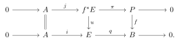
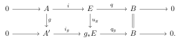
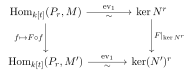
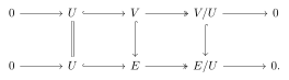
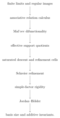
Read the complete exposition below, or download the matching 85-page PDF. Section and theorem numbers agree across the two editions.
Long study. The current programme enters at the commuting-operator calculus or transporter graph. The explicit relation construction recovers attachments; higher stabilization and cotangent theorems remain reference material.
Choose a complete reading route
In this exposition
An invertible replacement proves equality of finite basis sizes. A relation between two groups gives another working object: quotient its two ambiguities, and the relation becomes a canonical isomorphism. We perform both calculations before isolating their reusable operations in an exact Mal'cev setting. The resulting comparison proves refinement and Jordan–Hölder beyond the vector-space case.
Subsequent questions require different changes of working objects. Changing a lift measures a coupling coefficient; successive kernels recover nilpotent chains by finite differences; counting the same flags in two orders proves associativity. When orbit membership is insufficient, an action groupoid retains the actual moves. Later chapters construct linear coefficients over a nonlinear base and state the additional foundational inputs those questions need. Each route identifies the operation gained, its proof, and the data it cannot determine.
How to work through the constructions
Start with a question and the operation that changes it. Section 1 uses invertible replacements to prove equality of finite basis sizes. It then constructs a group comparison directly: keep a subgroup of a product as a relation, calculate the ambiguity on each side, and obtain a map between the quotients. Both are complete arguments before the general categorical definitions enter.
The common comparison route asks what those calculations used. Matching equations, forgetting witnesses, and quotienting compatible relations become explicit operations. The Mal'cev condition captures the three-corner calculation already performed in groups. Sections 2 through 4 develop refinement and compare its group and module instances.
Other questions have their own entry points. In Section 9, try changing a vector to remove an operator's coupling term; the calculation motivates the marked data subsequently classified. In Section 10, calculate successive kernel sizes and recover chain counts by finite differences; the chapter then constructs the chains that justify the calculation. In Section 11, count submodules and flags to obtain a product and prove its associativity. These are different operations, with different hypotheses and payoffs.
The final part is a further choice, motivated by a changed question. Section 12 begins with the moves that an orbit set forgets and retains them as arrows. Section 13 proves why a full additive replacement of groups cannot work, then constructs linear coefficients over a retained base. The stated higher-categorical equivalences are imported inputs; their role is identified where they are used. They are not prerequisites for the earlier finite arguments.
The theorem labels and dependency record identify the assumptions used in each calculation.
Part I · Construct the moves and the comparison
1 · Exchange vectors and remove ambiguity
When we write and then , something more organized than symbol manipulation is happening. We have applied an invertible map. When we then write , we have used a map that preserves an operation. These two ideas—invertibility and preservation—will remain visible as the objects become more general.
1.1 · Invert the move, then reuse it
Let be an abelian group. For , translation is the map of sets , . Associativity, the identity law, and the inverse law give
The same calculation in the other order proves . Thus means , and solving for means applying the inverse. Translation need not preserve the zero element, so it is generally an isomorphism of sets, not an automorphism of abelian groups.
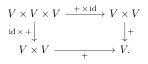
Associativity itself says that two composites are the same map:
Here the usual canonical identification of the two parenthesizations of the triple product is understood. The diagram says that making one intermediate sum rather than the other does not change the result.
If is another abelian group and preserves addition, then : the equality can be translated by . Also , because . Consequently
For a module, multiplication by a scalar is an additive homomorphism, so distributivity is exactly this preservation statement. In a group, the same discussion uses multiplication and left or right translations, with the order retained. Its multiplication is a map of underlying sets; it is not generally a homomorphism from the product group.
There is also a structural explanation of the triangular substitutions used in basis exchange. Given an additive homomorphism , the shear
has inverse . This follows by composing the maps, without counting any basis. Over a field, if , the map
is a scaling in the first coordinate followed by the shear on , where
Both maps are invertible. The inverse of the composite sends to and to for . This establishes the elementary maneuver without presupposing invariance of dimension.
We can already finish the basis-size question using this operation. Suppose is a basis and is an independent list. Express in the -basis. A nonzero coefficient gives a pivot; after permuting the 's, the invertible triangular substitution just constructed replaces by and leaves a basis. Express in that new basis. Some coefficient outside the fixed first vector must be nonzero, since otherwise would belong to the span of . Use that coefficient as the next pivot, fixing .
Continue in this way. After steps the first entries are , and the entire list is still a basis because every replacement was invertible. If , then after steps the next would be a combination of the preceding 's, a contradiction. Hence . For two bases, reverse their roles to obtain . Thus , without determinants, a dimension function, or a Jordan–Hölder theorem. The zero-space case gives two empty bases.
Later we obtain another proof from quotient comparisons. That proof will show how a similar comparison works when scalar pivots are unavailable; it is not needed to make this first argument complete.
1.2 · Remove ambiguity before choosing an output
Before introducing the language for a common comparison, perform one complete comparison in groups. Let be a subgroup of . Interpret as saying that is related to . Put
and record the ambiguities at the identity:
The sets are subgroups because products and inverses can be taken coordinatewise in . If and , choose ; conjugating by proves . Thus is normal in , and the same calculation proves that is normal in .
Try to send to a related . This need not give a map, because may not be unique. But if , their relative difference is , so . And if with , then . The assignment
is therefore well defined. Multiplying two related pairs proves that it preserves multiplication. It is onto by the definition of . If , multiply by to obtain , so . Hence its kernel is trivial and it is injective. We have constructed the comparison isomorphism directly.
The decisive operation is relative difference. For example, three pairs force the fourth because
Thus a relation that need not be a function becomes a function after quotienting exactly the ambiguities on its two sides. The following definitions isolate the matching, forgetting, and quotient operations so that the same proof can be used for other algebraic objects. A reader concerned only with groups can keep the displayed formulas as the working model.
A category consists of objects, sets of maps between objects, identity maps, and associative composition. A diagram commutes when every indicated pair of composites with the same endpoints agrees. A map is a monomorphism if implies ; a map is an epimorphism if implies . These are cancellation conditions on maps, not definitions in terms of elements.
A subobject of is a monomorphism into , with two such monomorphisms identified if an isomorphism over relates them. We write when the map representing factors through the one representing . Products are characterized by their projections: a map to is uniquely a pair of maps to and .
Definition 1.1 (Pullback).
For and , a pullback is an object with maps , such that , universal with that property: every pair , with has a unique map satisfying and .
We write .
In sets this is the set of pairs with the same image in . In groups and modules it has the same description with coordinatewise operations. The universal property retains the equation , without selecting coordinates. A terminal object receives exactly one map from each object. An initial object has exactly one map to each object. An equalizer of is universal among maps with . A finite-limit category has a terminal object, finite products, and equalizers, hence all the pullbacks used here: is the equalizer of . The kernel pair of is : it records exactly which inputs identifies.
A coequalizer of is a map with such that every map satisfying factors uniquely as . A regular epimorphism is a coequalizer of some pair. Every regular epimorphism is an epimorphism, by the uniqueness part of this property. We draw it as .
Lemma 1.2 (The elementary descent rule).
In a category with pullbacks, a regular epimorphism is the coequalizer of its kernel pair. It has the following lifting property against any monomorphism : in a commutative square
there is a unique with and .
Proof.
Choose a pair of which is a coequalizer. Since , this pair factors through the kernel pair of . A map equal on that kernel pair is therefore equal on , and descends uniquely through . This proves the first claim.
For the square, , and monicity of gives . Hence for a unique . Now , so because is epic. The equation also proves uniqueness.
□
In particular, a regular epimorphism that is also a monomorphism is an isomorphism: apply the lifting property to its square with itself and identity maps. This argument uses neither a choice of representatives nor a splitting assumption.
Definition 1.3 (Regular category).
A category is regular if it has finite limits, every map factors as a regular epimorphism followed by a monomorphism, and pullbacks of regular epimorphisms are regular epimorphisms. The monomorphism in
is called the image of .
Lemma 1.4 (Image calculus).
In a regular category, images are unique as subobjects, regular epimorphisms compose, and pulling back an image factorization gives an image factorization.
Proof.
Given two regular-epimorphism–monomorphism factorizations of a map, Lemma 1.2 gives a map between their middle objects in each direction. Its uniqueness says the two composites are identities. This proves uniqueness of images.
The lifting property in Lemma 1.2 is preserved under composition: first lift against the first regular epimorphism and then against the second. Factor their composite as , where is a regular epimorphism and is monic. The lifting property of the composite, applied against , gives a right inverse of . A monic map with a right inverse is an isomorphism. The composite is therefore a regular epimorphism.
Pull back the mono part of a factorization, and then pull back its regular epi part. The resulting square is a pullback of the composite, by the defining universal properties. Pullback stability makes the first part a regular epimorphism; pullbacks of monomorphisms are monic because maps into the pullback are determined by their two projections. This is the required image factorization.
□
Images express what survives a map. Pullback stability says that this description remains valid after imposing a compatible condition at the target. It is the reason local witnesses can safely be used below.
1.3 · A precise license to reason with witnesses
An arbitrary category may have too few maps from its terminal object to detect equality. In particular, a group has just one group homomorphism from the trivial group. Thus an argument about ordinary global points would miss nearly everything. We instead use generalized elements: an input of over a test object means a map .
For a subobject , saying that belongs to means that factors through that monomorphism. A cover below means a regular epimorphism, not an assumed topological covering.
Lemma 1.5 (Local witness calculus).
Let be a map in a regular category. A generalized element belongs to if and only if there is a cover and a map such that . Finite lists of such witnesses can be chosen over a common cover. They can be pulled back along any map of test objects.
Proof.
Factor with regular epic and monic. If , pull back along . The pullback cover has a map with . Conversely, such give a square against ; Lemma 1.2 makes factor through .
Pulling back a cover gives a cover. To combine two choices over , take their fiber product over ; either projection is a cover, and its composite to is a cover by Lemma 1.4. Repeat for finitely many choices. Nested choices are handled by composing covers.
□
This is the precise meaning of “there exists” in our relation calculations. A witness may exist only after a cover of the test object. Every proof using witnesses below permits that replacement. Equalities of subobjects are checked by inclusions in both directions: to check , one may test the generalized element itself. The method therefore proves actual categorical statements, not merely assertions about points.
1.4 · Relations compose by matching, then forgetting
Definition 1.6 (Internal relation).
A relation is a subobject of . Choose a representative with projections
The pair is jointly monic. We may write for membership in this subobject. Its opposite interchanges the projections. The identity relation is the diagonal .
If has carrier , form and take its image in . This is the composite . Thus
Our convention is always that means first , then . The pullback retains the matching intermediate value; the image forgets which matching value was used.
Proposition 1.7 (The calculus of relations).
In a regular category, relation composition is associative and has the diagonal relations as identities. It preserves inclusions, and
Proof.
For , , and , membership in either or means that, over a cover, there are with , , . Lemma 1.5 combines any nested witnesses into one cover and also allows the same triple witness to be grouped in either order. This proves equality of the two image subobjects. Equivalently, both are the image of in .
A diagonal intermediate relation forces the two matched coordinates to agree and introduces no further condition; hence the unit laws. An inclusion of relations sends every witness to a witness, proving monotonicity. Reversing a witness exchanges its endpoints and reverses the order of the two conditions, proving the last identity.
□
This associativity has the same shape as elementary reassociation, but it applies to correspondences that may not be functions. Its proof identifies one object of complete witness data and shows that the order of forgetting intermediate information does not matter.
A map is identified with its graph relation, represented by . The opposite graph is generally not a map: it remembers all possible preimages.
Lemma 1.8 (Graphs, kernels, and supports).
For a map ,
Here is the kernel pair, and the second diagonal is supported on the image subobject of . Consequently
Every relation with projections , satisfies
Proof.
The first composite relates exactly when , which is the defining pullback. The second relates exactly when, locally, for some ; this is the image diagonal by Lemma 1.5. These descriptions give the two consequences. Finally is the image of in ; that pair already represents the subobject .
□
Lemma 1.9 (When a relation is a map).
A relation is the graph of a unique map if
The first condition says that every input has a locally available output; the second says that the output is unique.
Proof.
Write with carrier . The first condition says that the image of is all of , so is regular epic. If have , then and are two outputs for the same input. The second condition gives . Joint monicity of gives , so is also monic and hence an isomorphism. Now has graph . Its value is forced by that graph, which proves uniqueness.
□
1.5 · Exactness makes an identification into an object
A relation is reflexive if , symmetric if , and transitive if . An internal equivalence relation has all three properties. Reflexivity also gives , so an equivalence relation satisfies .
Kernel pairs are equivalence relations. For example, transitivity says that and imply ; this is equally an equality of maps over any test object.
Definition 1.10 (Barr exactness).
A regular category is Barr-exact if every internal equivalence relation is the kernel pair of a map. Equivalently, for every such on there is a regular epimorphism with . We call the quotient .
For the equivalence of these formulations, factor a map exhibiting the kernel pair into its image. The monomorphism part does not change its kernel pair, and the other part is regular epic. Lemma 1.2 then gives the quotient's full universal property: maps from that identify the pairs in descend uniquely to . Two such quotients are uniquely isomorphic over , by applying this property twice. Exactness concerns these equivalence-relation quotients; it does not assert that the category is abelian or that its maps can be added.
A category is pointed if it has an object that is both initial and terminal. There is then a zero map between every two objects, namely the composite through . A kernel of is the pullback of along :
The left map is monic since is monic. In a pointed category it is a distinguished subobject, but it is only one class of the whole kernel pair.
If , its zero class is the relation , viewed as a subobject of , where . Since ,
It is saturated: . We will retain both the full equivalence relation and its zero class. In groups the zero class determines the normal quotient, but we will not build that additional fact into the general framework.
The roles of the assumptions are now visible. Finite limits impose compatible equations. Images forget witnesses. Regularity makes that forgetting compatible with substitution. Exactness realizes consistent identifications as quotient objects. Pointedness selects a zero class. The next condition will make different identifications compatible with one another.
2 · The three-corner rule and one comparison
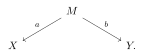
Suppose a relation connects inputs in with outputs in . Three corners of a rectangle may already force the fourth:
This property is called difunctionality. It says that the relation breaks into complete rectangular blocks. It does not say that each input has just one output. Several inputs and several outputs can belong to the same block.
The structural comparison is already suggested by this picture. Group the inputs according to which block they occupy, and group the outputs in the same way. The two resulting quotient objects should agree. We will construct that agreement, including its maps, before using it to compare any filtrations.
2.1 · Why relative difference is enough
Definition 2.1 (Mal'cev category).
A regular category is a Mal'cev category if every reflexive internal relation is an equivalence relation.
This categorical condition has an elementary source. Suppose we have algebraic structures with a ternary term satisfying
If a compatible relation is reflexive and , its closure under gives
Thus it is symmetric. If also , closure gives
so it is transitive. The operation is applied coordinatewise to pairs. For groups ; for modules it is . No commutativity of group multiplication was used. A term is an operation on the underlying algebra; in the group case it need not be a group homomorphism from to .
The group calculation in Section 1 used precisely this move: take a relative difference, then reattach it at another point. In a module the corresponding calculation is . The categorical condition records the rectangle-completion effect shared by these calculations. The next proposition proves that it supplies the same reusable rule even when there is no chosen formula for relative difference.
Proposition 2.2 (Three forms of the Mal'cev condition).
For a regular category the following conditions are equivalent:
every reflexive relation is an equivalence relation;
equivalence relations on the same object commute under relation composition;
every relation is difunctional, that is,
Proof.
Assume the first condition. If are equivalence relations on , their composite is reflexive, since both contain . It is therefore symmetric, and
This proves the second condition.
Assume the second. Give a carrier with projections and . The kernel pairs
are equivalence relations on the same object , so they commute. Using Lemma 1.8, we obtain
The equalities are typed on ; we have not interchanged unrelated relations on and . This proves the third condition.
Finally assume the third and let be reflexive. Monotonicity gives
Taking opposites gives the reverse inclusion, so is symmetric. Also , and hence . Thus is transitive and is an equivalence relation.
□
The local-witness interpretation of is exactly the three-corners implication above. The reverse inclusion always holds: a related pair can supply all three edges of a degenerate rectangle. The proposition explains why the rectangle-completion law holds simultaneously for every relation, rather than having to be verified anew for each quotient comparison.
2.2 · Partial identifications and their supports
Relations used in a filtration may live on a subobject rather than all of the ambient object. We must record that support instead of silently assuming reflexivity everywhere.
Lemma 2.3 (Partial equivalence relations).
Let be symmetric and transitive in a regular category. The two projections of its carrier have the same image . Restricted to , the relation is an equivalence relation . In a Barr-exact category there is a regular epimorphism with
Conversely, every relation of this displayed form is symmetric and transitive, with support .
Proof.
Symmetry interchanges the two projections, so their images agree. Their factorizations through give a relation ; the pair is still jointly monic. Both of its projections are regular epic. If is an input in , a cover supplies a witness . Symmetry gives , and transitivity gives . Lemma 1.5 descends this membership, so is reflexive. Symmetry and transitivity are inherited by restriction. Exactness gives , proving the formula.
Conversely, is an equivalence relation on . Its extension along is symmetric; since , its square is itself. The projections onto are regular epic because the relation is reflexive, so their images in are .
□
We call the quotient of the partial equivalence relation. It is the quotient of its support, not a quotient of all of . This distinction permits the same relation language to describe every step of a chain whose terms are only normal in their successors.
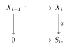
For example, a quotient map with determines a relation on : two inputs are related precisely when they both lie in and have the same image in . Its support is ; in a pointed category its zero class is . Thus one partial relation remembers the numerator, the identifications, and the chosen quotient, up to its unique quotient isomorphism.
2.3 · One relation, two quotients, one object
Let have carrier and factor its projections through their images:
The pair is jointly monic. We use for the relation on these supports, so . Both projections of are regular epic.
Theorem 2.4 (The universal support-quotient comparison).
In a Barr-exact Mal'cev category, put
These are equivalence relations. For their regular quotient maps and , there is a unique isomorphism satisfying
In particular the two support quotients of any relation are canonically isomorphic.
Proof.
Because is regular epic, every input in has locally some -related output. Using that same output twice proves . Likewise . Both relations are symmetric by taking opposites. Difunctionality gives
Thus they are equivalence relations, and exactness supplies .
We construct the map rather than merely matching equivalence classes. The map is equal on the kernel pair of : if , then and share a -related input, so they are -related and . Lemma 1.2 gives a unique with .
Next is equal on . An -related pair is locally of the form with . Consequently . These equalities hold after a cover, and covers are epimorphisms, so they hold on the relation itself. Hence descends uniquely through , giving .
The same construction with the opposite relation gives such that . It follows that
Both and are composites of regular epimorphisms, hence are epic. Cancellation proves and . Finally is epic, so the equation specifying proves its uniqueness.
□
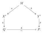
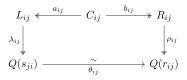
The construction is summarized by the commutative diagram
There is generally no map to put across the middle row. The relation supplies multiple possible outputs. The quotient removes precisely their ambiguity, after which the comparison becomes a uniquely determined isomorphism.
For a familiar model, take the additive group and the relation meaning that is even. This is a subgroup of , with both supports equal to . Two inputs share an output precisely when they have the same parity; the same is true of two outputs sharing an input. Thus both support quotients are , and the comparison sends the parity class of an input to that of any related output. There are infinitely many possible outputs before quotienting, but exactly one class afterwards. This illustrates the construction; the categorical theorem did not need a preferred output or a choice of representatives.
Here is another view of the same map, useful for computations. Its graph is
Indeed,
We used , , their idempotence, and , . Lemma 1.9 makes a map, and makes its inverse. This is the same because its graph relates the quotient images of every pair in .
This theorem is the comparison mechanism from which the refinement rectangle will be built. It is stronger than a statement about lengths: it constructs the actual isomorphism between the surviving objects. No filtration, simplicity assumption, or Jordan–Hölder theorem has entered its proof.
2.4 · Which relations descend through a quotient?
There is one further compatibility to make explicit. If we identify inputs by a quotient map, a relation descends only when changing an input within its equivalence class does not change the relation. This is saturation.
Proposition 2.5 (Saturation and descent).
Let and be regular epimorphisms, with kernel pairs and . There is an order-preserving bijection
It sends to , and its inverse sends to . The first construction is precisely inverse image of the relation along .
Proof.
Inverse image consists of pairs whose quotient images satisfy , which is by the graph formulas. Since and , the two constructions satisfy
An inverse-image relation is saturated because and . Thus the formulas are mutually inverse exactly on the stated saturated relations. Both are order preserving by monotonicity of relation composition.
□
For a relation on and a single quotient , saturation is . Since contains the diagonal, this implies separately and . Consequently the correspondence respects composition of saturated relations:
It also respects opposites. Thus a saturated symmetric transitive relation descends to a symmetric transitive relation, including its possibly proper support. Conversely, inverse image preserves these properties: for example
when is transitive. These statements hold for partial equivalence relations as well as for equivalence relations on all of .
Corollary 2.6 (Quotients of quotients).
In a Barr-exact category, fix with kernel pair . Equivalence relations on correspond to equivalence relations on containing , by
If is the quotient of , it factors uniquely as , where is the quotient of . Thus , with the isomorphism determined by the quotient maps.
Proof.
If is an equivalence relation containing , then , so it is saturated. Its descent is reflexive because , and is symmetric and transitive by the preceding formulas. Conversely, the inverse image of an equivalence relation is an equivalence relation containing .
Since , the map is equal on the kernel pair of , so it descends uniquely to . Factor into its image. If its mono part were a proper subobject of , then would factor through that same subobject, contradicting the lifting property of the regular epimorphism . Hence is regular epic. Its kernel pair is
Lemma 1.2 makes it the quotient of . The universal property proves the claimed canonical isomorphism.
□
This last result needs exactness and regularity, but not the Mal'cev condition. Recording that distinction matters: Mal'cev is used to make every relation difunctional and hence to produce the universal comparison. The ordinary law for compatible iterated quotients has already been supplied by exactness. Later, in a higher setting, we will see why retaining such compatibility data remains essential.
The relation calculus and support comparison are classical. For context, see Knop, Tensor envelopes of regular categories, Section 5 and Appendices A–B. The arguments here have been written out so that the refinement theorem can depend on explicit constructions rather than on an unnamed isomorphism theorem.
3 · A quotient remembers which identifications were made
We now have a language in which a quotient is an operation on a relation, and a comparison of quotients is an operation on a correspondence. We will use that language once, in a pointed Barr-exact Mal'cev category . Groups and modules will enter afterwards by verifying these axioms. Neither commutative addition of arrows nor an invariant called dimension is used in this chapter.
There are three stages. First we record a normal series without forgetting its quotient maps. Next we compare two such records by a rectangular array of correspondences. Finally simplicity prevents the comparison from breaking a factor into smaller nonzero factors. The last step is Jordan–Hölder; the rectangle, rather than a numerical count, does the work.
3.1 · The data in a normal series
Definition 3.1 (Normal series with its quotient maps).
A finite normal series of consists of a chain of subobjects and chosen regular epimorphisms
such that the inclusion is a kernel of . The objects are its factors. Repetitions of subobjects and zero factors are permitted. Two series are equivalent when their lists of factors are isomorphic after a permutation. We also use equivalence after deleting zero factors, stating explicitly when we do so.
It is a pullback. In particular, the normality assertion is relative to , not to all of . For a group this allows a subgroup normal in its successor without demanding that it be normal in the ambient group.
We keep because the kernel alone need not determine a quotient in this generality. A familiar implication from groups, such as “a regular epimorphism with zero kernel is an isomorphism”, is not inserted as an unstated axiom. All our comparisons retain the kernel pair of the actual map, which is the full record of its identifications.
Here and below, composition of relations is function-like: means first , then . For a relation and a subobject , write for the image of the restriction of whose input lies in . Thus is its output support and its zero class. A symmetric transitive relation is a partial equivalence relation; it is an equivalence relation on its support, by Lemma 2.3. Its support quotient will be written
The slash is shorthand for the effective quotient of the restricted equivalence relation, not a new operation on objects without relations.
Lemma 3.2 (A series as a sequence of identifications).
For , the data of Definition 3.1, up to the unique isomorphisms allowed for quotient objects, are equivalently a list of partial equivalence relations on satisfying
(1)
The associated factors are . The empty series of is treated separately; it has no endpoint relations to name.
Proof.
Let be the composite inclusion. Regarding arrows as their graphs, put
On , this is the kernel pair of ; it relates precisely the two inputs that identifies. Extending it along the monomorphism makes it a partial equivalence relation on . Its support is . The zero arrow into is sent to the zero arrow into , so taking the zero class of that kernel pair gives precisely the pullback defining . Therefore
These equalities give (1). Since is a regular epimorphism, it is the effective quotient of its kernel pair, and canonically.
Conversely, set . The zero class is a subobject of . Thus the identities (1) make the a chain, beginning with and ending with . By exactness the restricted relation has an effective quotient . The same kernel-pair calculation says that . These two constructions are inverse because an effective quotient is determined, up to a unique compatible isomorphism, by its kernel pair.
□
This change of language has retained more than the chain. It retains which pairs of points become equal at each step. That is the information needed to compare two quotient constructions in a category where the zero class alone may not determine the entire relation.
3.2 · What a genuine refinement means
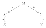
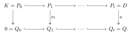
To refine a series, we refine one of its factors and pull that refinement back. Suppose is one quotient step, with kernel , and suppose
is a normal series of its factor. Form . We obtain
Each displayed comparison square is a pullback. Pullback stability of regular epimorphisms makes a regular epimorphism. The refined quotient map at the th step is
(2)
Its kernel is : its pullback over is . Regular epimorphisms are closed under composition, so this really is a normal series between and . Replacing any or all of the original steps in this way is what we mean by a refinement. For the empty series of the zero object we adopt the harmless convention that inserting a finite list of zero steps is a refinement. This convention concerns only how empty lists are represented; it introduces no nonzero factor.
It would be insufficient to insert arbitrary kernel subobjects between and while forgetting their relation to . We need the new quotients to have arisen from the original quotient. The following saturation condition expresses exactly that requirement.
Proposition 3.3 (Saturation is descent of a refinement).
Let be a partial equivalence relation on , let , and let be its quotient. For , lists of partial equivalence relations on satisfying
correspond to normal series of with exactly steps. Under this correspondence, their support quotients are the factors of the pulled-back refinement of .
Proof.
The equality first implies that the support of lies inside , so we can work on . Write for the kernel pair on ; it is the restriction of . The saturated descent lemma, Proposition 2.5, gives mutually inverse operations
The first is the direct image relation on ; the second is its pullback along . Their being inverse uses and . That lemma also proves that symmetry and transitivity descend, so each is a partial equivalence relation.
We check the endpoints, since those checks are what make this a descent of series. Saturation and reflexivity of on give . The inverse image of the zero subobject of is . Therefore, as subobjects obtained by regular images,
In the other direction, begin with a normal series of and its relations . Pulling back the relations gives , which are saturated and have precisely the support and zero-class boundaries in (4). Concretely, if is the support of , the support of is . If is its factor quotient, the kernel pair of on is . As is a regular epimorphism, its codomain is the effective quotient of . This gives the unique compatible isomorphism and identifies the quotient maps as well as the objects.
□
The proposition is a small descent theorem. The equality says that changing either input by an identification already imposed by does not change the new relation. Exactly then the relation can be defined downstairs, independently of the choice of a representative. The proof above replaces that verbal test by pullbacks, images, and unique quotient maps.
3.3 · The comparison rectangle
Let be partial equivalence relations on the same object. Their composite need not be an equivalence relation on all of . It is nevertheless a relation, so the Mal'cev theorem applies to it. This produces the identities that will make our rectangle fit together.
Lemma 3.4 (Two endpoint identities).
For partial equivalence relations on ,
(5)
and
(6)
Proof.
The relation is difunctional by Proposition 2.2, so . Symmetry and idempotence of reduce the left side to
Every subobject in a pointed category contains its zero arrow. In particular and . Monotonicity of relational image and (5) now give
Here the second inclusion comes from , itself obtained by applying to . For supports, gives
the final inclusion uses . Both chains give equality.
□
Now take two normal series of of positive lengths , encoded by and . At the crossing of the th row and th column, define
(7)
The two cell relations are the two equivalence relations associated with the correspondence :
Our composition convention matters here: is on the input support of , and on its output support.
Proposition 3.5 (Every row and column is a genuine refinement).
For fixed , the list satisfies Proposition 3.3 for . For fixed , the list satisfies that proposition for .
Proof.
We verify every condition for a row. Symmetry follows by reversing the word . Idempotence follows from Lemma 3.4:
Thus each cell is symmetric and transitive. Its saturation is
For the first zero class, use :
For an intermediate join, use :
For the last support, use :
Every equality that removes the trailing is one of (6). We have proved saturation and all boundary conditions, so Proposition 3.3 supplies a pulled-back refinement of the original quotient. Interchanging and proves the column assertion.
□
The boundary identities are the gluing conditions. They say that the support of one cell is precisely the zero class required to start the next cell. Without these identities we would have an assortment of quotients, not a refinement of a filtration.
Proposition 3.6 (The two readings of a cell have the same quotient).
For every there is a canonical isomorphism
(8)
It is induced by the correspondence and characterized by its two projections, not chosen by comparing lengths or other invariants.
Proof.
Let be the object representing . Factor its two projections through their image supports:
Both and are regular epimorphisms. The input relation is , so ; similarly . Write their effective quotient maps as and .
The support-quotient comparison theorem, Theorem 2.4, applies to and gives the unique isomorphism for which
commutes, meaning . The cited theorem proves existence and invertibility by effective quotients and difunctionality. Its uniqueness also follows directly because is an epimorphism. The displayed computation of the two kernel relations identifies its conclusion with (8).
□
This is the categorical butterfly. It is the same correspondence read from its two ends, with each end quotiented by precisely the ambiguity introduced by that correspondence. No picture of four wings is needed to remember the construction: form , compute and , and take their support quotients.
Theorem 3.7 (Schreier refinement in an exact Mal'cev category).
In a pointed Barr-exact Mal'cev category, any two finite normal series of an object have equivalent refinements in the pullback sense specified above. The refinements may contain repeated subobjects and zero factors.
Proof.
Suppose first that both series have positive numbers of steps. For the first series, concatenate the rows supplied by Proposition 3.5. Their endpoints are the original successive subobjects, so they fit together into a normal series of . For the second series, concatenate the columns. Both refined lists have factors. Their indexing orders differ, but the transposition pairs them. Proposition 3.6 gives the isomorphism for each paired cell.
An empty series can occur only for . Every subobject of is isomorphic to : a monomorphism has its unique map as a right inverse, and monicity makes it a left inverse as well. A regular epimorphism out of also has zero codomain, since it is at once monic and a regular epimorphism. Thus every factor of every series of is zero. We may insert zero steps to give both series the same positive number of zero factors, or treat two empty lists as already equivalent. These are refinements by the zero object's zero series. This resolves the degenerate case without assuming a nonempty comparison rectangle.
□
The theorem does not produce a single nested chain containing the terms of both original chains. Two different lines in a two-dimensional vector space already prevent that: neither line contains the other. It produces one refinement of each chain and a matching between their quotient factors. This distinction matters even in the most elementary example.
3.4 · Simplicity removes the remaining freedom
Definition 3.8 (Quotient-simple object).
A nonzero object is quotient-simple if every regular epimorphism is either an isomorphism or has zero codomain. A composition series is a finite normal series all of whose factors are quotient-simple.
The condition concerns the arrow . The weaker phrase “its codomain is isomorphic to or to ” would not exclude a proper self-quotient. The definition above does exclude it. In the group and module instances, it agrees with the usual definition of a nontrivial simple object.
Lemma 3.9 (A simple factor cannot be broken into smaller factors).
Every finite normal series of a quotient-simple object has exactly one nonzero factor, isomorphic to . Its other factors are zero.
Proof.
The last quotient is a regular epimorphism . If , its kernel is all of , so the preceding subobject is . Remove this last, zero-factor step and consider the shorter series. Because the series is finite and begins at , this removal process must eventually reach a last step whose preceding subobject is proper in .
For that step the quotient cannot have zero codomain: a map to has kernel . Simplicity therefore makes the quotient map an isomorphism. Its kernel is , so every preceding subobject of the chain is . Every regular quotient of is , as checked in the proof of Theorem 3.7. We have one quotient isomorphic to , zero quotients before it, and the zero quotients stripped from its end.
□
Theorem 3.10 (Jordan–Hölder).
Let be a pointed Barr-exact Mal'cev category. If an object has two finite composition series, then their factor lists agree, including multiplicity, up to permutation and isomorphism. In particular, the two series have the same number of factors.
Proof.
Apply Theorem 3.7 to obtain equivalent refinements. Each refinement is obtained from normal series of the original factors, pulled back along the original quotient maps. By Lemma 3.9, each such factor series contributes exactly its original simple factor and some zero factors. Proposition 3.3 identifies these with the factors of the pulled-back refinement.
Consequently, deleting zero factors from the first refined list recovers the first original list, and deleting them from the second recovers the second original list. An isomorphism cannot identify a nonzero object with , so the matching between refined lists restricts to a matching between their nonzero lists. This is the desired permutation and set of factor isomorphisms. The equality of lengths is a consequence of that bijection, not an input to its construction.
□
No existence assertion is hidden in this theorem. We assumed two finite composition series and compared them. A category may contain objects with no finite composition series. Even when maximal or minimal subobjects can be selected, a termination argument is still required before one can assert existence. The finite sequences used here are already supplied, so neither an ascending nor a descending chain condition enters the uniqueness proof.
3.5 · Factor data becomes an invariant only after the comparison
Now, and only now, a numerical or algebraic record of the factors becomes legitimate. Call an object composition-finite when it has a finite composition series, allowing with its empty series. Write for the finite multiset of isomorphism classes of its simple factors. Theorem 3.10 proves that is independent of the chosen series. It does not reconstruct : distinct extension data can give the same multiset.
Proposition 3.11 (Splicing an extension).
Suppose is a regular epimorphism with kernel . If and are composition-finite, then so is , and
(9)
Here means disjoint union of finite multisets, including multiplicity.
Proof.
Choose composition series for and . Pull the series of back along . The construction (2) gives a normal series from to whose factors are exactly those of . Prepend the chosen composition series from to . Every factor in the resulting series is simple, so it is a composition series of . Its factor list is the concatenation of the two chosen lists. Jordan–Hölder makes that calculation independent of all the choices and proves (9).
□
This proposition establishes closure under these extensions. It does not assert, without an additional argument, that every subobject or every regular quotient of a composition-finite object is composition-finite in our weakest categorical setting. The direction used in the proof is precisely the direction stated.
For the next statement assume that the isomorphism classes of simple objects under discussion form a set , for example by working in an essentially small category. The free commutative monoid consists of finitely supported functions , with pointwise addition. Thus is an element of this monoid.
Corollary 3.12 (The universal additive record).
Let be a commutative monoid. An arbitrary assignment extends uniquely to an isomorphism invariant of composition-finite objects satisfying
for every kernel–regular-quotient sequence whose terms are composition-finite. The formula is
Proof.
Only finitely many summands are nonzero. Jordan–Hölder makes the formula well defined, and Proposition 3.11 gives the required additivity. For uniqueness, every intermediate term of a composition series is composition-finite, because its initial segment is itself a composition series. Repeatedly applying additivity to these successive quotient maps forces to equal the displayed sum.
□
Taking every defines length. Taking values in a group gives the corresponding universal group of additive invariants. These are consequences of factor comparison; using them to justify that comparison would reverse the dependency and create circular reasoning. The order here is deliberate: quotient construction, refinement, factor matching, then invariant.
3.6 · What is natural in the construction
Proposition 3.13 (Transport by a regular functor).
Let be a functor between pointed Barr-exact Mal'cev categories that preserves finite limits, regular epimorphisms, and a zero object. Then transports the relation rectangle, its refinements, and its cell isomorphisms to the corresponding constructions in , up to their canonical structural isomorphisms.
Proof.
Finite-limit preservation gives preservation of monomorphisms, products, kernel pairs, kernels, and pullbacks. If a map is factored as a regular epimorphism followed by a monomorphism, its image under is again such a factorization. Uniqueness of image factorizations therefore shows that preserves images. Relational composition is an image of a pullback projection, so identifies with . Converse relations are preserved by preservation of the product symmetry.
If is the effective quotient of an equivalence relation , then is a regular epimorphism and its kernel pair is . Hence it is the effective quotient of . These observations preserve every operation in (7), the support and zero-class equations, and the pullback squares defining refinements. Finally the image of the commuting diagram in Proposition 3.6 satisfies the same characterization as the cell comparison in . Its uniqueness identifies the two isomorphisms.
□
A regular functor need not preserve simple objects. For instance, forgetting a module's scalar action can reveal additive subgroups that were not submodules. The proposition transports the comparison construction; a statement about composition series additionally requires that the relevant simple factors remain nonzero and quotient-simple. This distinction prevents a change of framework from silently forgetting part of the theorem's information.
3.7 · Dependency and scope check
The ordinary categorical proof is now complete. The foundation needed finite limits and regular images for relation composition, exactness for the effective quotients, and the Mal'cev condition for difunctionality. Pointedness supplied zero classes and kernel boundaries. Saturated descent made each row a refinement of the chosen quotient map. The support-quotient comparison matched each cell. Simplicity then removed the zero cells. No invariant length, dimension, Grothendieck group, or pre-existing Jordan–Hölder theorem entered the chain of dependencies.
The comparison pattern is the classical categorical refinement argument associated with Lambek; Knop's Appendix B2 gives its exact Mal'cev formulation and emphasizes the saturation requirement. The proof here has supplied the descent, boundary, and quotient-map checks explicitly; it is not a claim of a new theorem. The detailed primary reference is Friedrich Knop, Tensor envelopes of regular categories, Appendix B2.
What has become general is a construction with stated hypotheses, not the assertion that every category has composition factors. The later homotopical chapters will ask which quotient and refinement data survive when equalities become coherent identifications. The present theorem is available there whenever its ordinary exact Mal'cev hypotheses are actually verified; it does not, by terminology alone, assert a Jordan–Hölder theorem for arbitrary higher objects.
Part II · Reuse the comparison and calculate its pages
4 · Groups, modules, and dimension as instances
The comparison theorem has been proved before choosing a multiplication table, a scalar field, or a basis. To use it, we must now check its hypotheses. This is an essential part of the argument: a category name does not by itself verify an image factorization or construct a quotient.
4.1 · One verification for algebraic structures
An algebraic theory specifies operations of finite arity and equations between expressions built from them. A model is a set with those operations satisfying the equations; a morphism preserves every operation. A subalgebra is a subset closed under them. An internal relation on a model is a subalgebra of . An equivalence relation of this kind is a congruence: equivalent inputs give equivalent outputs for every operation.
Proposition 4.1.
The category of models of an algebraic theory is Barr-exact. If its one-element model is also initial, it is pointed. If the theory has a ternary term satisfying
then it is a Mal'cev category. Under these last two conditions the general comparison theorem applies to its finite composition series.
Proof.
Products carry the operations coordinatewise. An equalizer is the subset where two homomorphisms agree, closed under every operation. These give finite limits, with the one-element algebra terminal. The image of a homomorphism is a subalgebra, so every map factors as a surjection followed by an inclusion. A pullback of a surjection is surjective: an element of the other object has a lift of its image, giving a pair in the pullback.
Let be surjective. A homomorphism constant on its fibers defines for any with . This is independent of , and choosing lifts of the finitely many inputs of an operation proves that preserves that operation. Surjectivity proves uniqueness. Thus is the coequalizer of its kernel pair.
Conversely a regular epimorphism is surjective. Factor a coequalizer through its set-theoretic image as . If coequalizes , injectivity of shows . Its universal property supplies with . Then , so because coequalizers are epimorphisms. Also , and the surjectivity of gives . Hence is an isomorphism. We have established regularity with exactly the stated quotient maps. Monomorphisms are precisely the injective homomorphisms: injectivity gives left cancellation, while factoring a monomorphism into its image makes the surjective part both monic and regular epic, hence an isomorphism by Lemma 1.2. Thus the internal subobjects and relations really are the subalgebras used in the next step.
For a congruence on , form the set and define every operation on classes by applying it to representatives. Closure of under the operation makes this well-defined; the equations descend because they hold on representatives. The quotient map has kernel pair exactly and has the same coequalizer property just proved. Thus every internal equivalence relation is effective, proving Barr-exactness.
Finally let be reflexive and an internal relation. It is closed under the term . If , apply to to obtain , proving symmetry. If and , apply to to obtain , proving transitivity. Thus every reflexive internal relation is an equivalence relation. The pointed assertion is precisely the extra initial-object hypothesis.
□
The displayed terms are operations in a presentation. For a nonabelian group, , , need not be a group homomorphism. What we used is that a subalgebra is closed under terms, including that term. This distinction lets algebraic expressions justify a categorical property without confusing them with arrows in the category.
4.2 · Reading the axioms in familiar examples
For groups use multiplication, inverse and identity, with their axioms. The one-element group is initial and terminal, and has the required identities. For left modules over a fixed unital ring , use addition, negative, zero, and an operation for every , with the module equations. The zero module is initial and terminal, and works. Neither argument uses a dimension, a composition series, or Jordan–Hölder.
We check that the categorical quotient data are the familiar ones. In a group , the kernel of a homomorphism is normal, since . Conversely, for a normal subgroup , the relation if is an equivalence relation compatible with multiplication and inverses. For example, if and , then differs from by an element of . The congruence quotient just constructed is the usual group .
More generally, if is a group congruence, its identity class is a normal subgroup: closure gives products and inverses, and conjugating a pair by gives . Translating by shows exactly when . Thus normal subgroups and these quotient relations agree.
For modules, a congruence has zero class a submodule , and translating pairs gives exactly when . The quotient operations are and . Consequently all isomorphisms supplied by the categorical theorem are -linear. A quotient-simple group is exactly a nontrivial group with no proper nontrivial normal subgroup; a quotient-simple module is exactly a nonzero module with no proper nonzero submodule.
We therefore obtain both classical theorems from Theorem 3.10: two composition series of a group have the same group factors, and two of an -module have the same module factors. This is one specialization step for each category, not a second proof of the comparison theorem.
The same verification covers groups with specified endomorphism operators: include those operators and their preservation equations in the theory. Subobjects and quotients retain them. It also covers Lie algebras over a field, using the additive term , and nonunital associative algebras over a commutative ring. Their kernels are respectively ideals and two-sided ideals. For Lie algebras our categorical use of simple includes a one-dimensional abelian algebra. Unital rings with identity-preserving maps do not have a zero object and are not a direct instance of this pointed statement.
4.3 · Reading one cell as the familiar group butterfly
Take and . Let be the partial equivalence relations on supplied by and . Put
Applying and then to a subset means taking the appropriate congruence classes inside and then inside . In particular, and , so the endpoint identities give
Here denotes the identity subgroup. Interchanging the two relations gives support and identity class for . Since a group congruence is determined by its identity class, the two cell quotients are
We can see their common quotient and every normality assertion directly. The groups are normal in : conjugation by an element of preserves or , respectively, and remains in the other ambient subgroup. Consequently is a normal subgroup of . The product is a subgroup because and . In , the image of is the whole group and the image of is normal. Its inverse image is , proving . The same argument proves .
Now use the two homomorphisms
Both are onto, since the extra factor or is killed. The first kernel is : if lies in , then ; the converse inclusion is immediate. The second kernel is , by the same calculation. The effective quotient property therefore gives
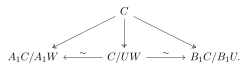
These isomorphisms give the usual butterfly, with its maps specified. They are also the previously constructed cell comparison: for every element of the correspondence , its two ends can be represented as and , with , and . Both quotient maps then use the same class of . The characterization in Proposition 3.6 identifies the maps. Thus the subgroup products are the concrete supports and identity classes of one categorical construction.
4.4 · A comparison that changes the order
In put and . Reduction modulo has kernel and reduction modulo has kernel . Hence
have factors and . Every nonzero element of or generates the group, so the factors are simple. The relation comparison becomes the following concrete rectangle:
Indeed and , since modulo . The two nonzero comparisons are induced by and . Each is onto by the sum equality and injective by the intersection equality. These are actual isomorphisms, not just equalities of cardinalities. A refined chain need not contain both and ; the matching occurs between its factors.
Normality is always in the next term. In , for example, has both terms normal in the ambient group, but is not simple. Insert one of its order-two subgroups to obtain a composition series. That subgroup is normal in the abelian group and is not normal in : conjugation by a three-cycle permutes the three double transpositions. The lattice of subgroups normal in the ambient group describes a different filtration problem.
4.5 · Finite basis size, with no dimension in the prerequisites
Let be a field. A list is a basis if it spans the vector space and every relation has all . The module construction above provides subspaces, quotient spaces and their linear maps before any notion of dimension is introduced.
Theorem 4.2 (Invariance of finite basis size).
If has finite bases and , then .
Proof.
Put , with . Each inclusion is strict: otherwise would be a linear combination of the preceding vectors, contradicting independence. The map
is onto by the definition of span. If its image is zero, a relation with coefficient on shows . It is therefore an isomorphism of -modules. The module is simple: a submodule containing contains and every scalar multiple of . The basis thus supplies a composition series with factors isomorphic to . The other basis supplies one with factors. Apply the general Jordan–Hölder theorem in -modules. If , independence forces both lists empty, giving the same conclusion.
□
The direct exchange proof in Section 1 already established this equality by successive invertible replacements. The proof here obtains it from comparisons between quotient layers. The extra work has a different payoff: it explains why the comparison survives in algebraic settings without scalar pivots. Neither argument uses a pre-existing dimension function. We may define using their common conclusion, then develop rank–nullity and other finite-dimensional operations without circularity.
4.6 · What a factor list leaves unresolved
Both and have factors . Their exact sequences can be written
where the last two maps in the second sequence are first-factor inclusion and second-factor projection. The first quotient is reduction modulo . The displayed kernels and surjections verify exactness directly. Yet has an element of order four, whereas every element of is killed by multiplication by two. They are not isomorphic. The general theorem compares the simple pieces. It does not split the extension joining them. The following parts develop measurements and constructions that retain more of this attachment information.
5 · Keeping the operations when we change the object
The common comparison has produced intrinsic simple factors. Its group example also showed a limit: the factors of and agree, although the groups do not. We now develop that question in a setting where the attachments can be calculated explicitly. The objects will be modules, and our main examples will be vector spaces equipped with an operator. We retain the operator in every map, just as the dimension argument retained scalar multiplication in every quotient.
5.1 · Modules and their maps
A ring has an abelian group under addition, an associative multiplication with identity , and the two distributive laws. Multiplication need not be commutative. A left -module is an abelian group with operations for , , satisfying
The same cancellation arguments as for vector spaces give , and . A submodule contains zero and is closed under addition and all these scalar operations. A module map preserves addition and satisfies . In this part all unspecified maps between modules are module maps. We work over a fixed ring whenever forming extensions or comparing modules.
Intersections of submodules are submodules. Their sum consists of the elements ; distributivity proves that it is a submodule, and it is the smallest one containing both. The direct sum of two modules is the set of pairs with coordinatewise addition and scalar action. Each module identity holds in both coordinates. Its inclusions and projections are module maps. A map out of is determined by its restrictions to and , since .
For a submodule , the additive quotient is already defined by the group construction. Set . Replacing by changes by , so this action is well-defined; the module identities descend on representatives. The projection is a module map. If a module map kills , its unique additive factorization is a module map, because
Thus the quotient universal property retains every operation required here.
Kernels, images and preimages of submodules are submodules: apply a map to a sum or a scalar multiple, and use the corresponding closure in the target. An image of a submodule is the image of the map restricted to it. Consequently the first isomorphism theorem supplies a module isomorphism
The inverse of a bijective module map is a module map: writing gives , and the analogous calculation handles sums. All the short exact sequences below mean injectivity, surjectivity, and image equal to kernel for these maps.
5.2 · Preimages, quotients, and the local comparison
For a surjection with kernel , inverse image and direct image give an inclusion-preserving correspondence between submodules of and submodules of containing . Indeed, for a submodule of ,
Every quotient map and induced isomorphism in this correspondence is linear over . For this also proves by .
The kernel calculation at the heart of the butterfly remains valid: if and are submodules of , write , , . The map
is onto, and its kernel is . To check the nontrivial inclusion, if with and , then . The reverse inclusion follows by substitution. Exchanging and gives the same kernel and the other wing. This is a concrete calculation of the common support quotient, retaining the -action. It is available independently of any theorem about composition series.
5.3 · Finite-dimensional tools, after dimension has been proved
The later operator examples use subspace bases and lifts. We establish their existence here, after Theorem 4.2; none is being fed back into the earlier proof of dimension.
Lemma 5.1.
If a vector space has a finite basis of size , every subspace has a finite basis. Every independent list in extends to a basis of . For a subspace , a basis of followed by lifts of a basis of is a basis of .
Proof.
Start with any finite independent list. Pass through a fixed finite spanning list of , appending a vector exactly when it is outside the span of the vectors already present. Each append preserves independence: a relation with nonzero coefficient on the new vector would put it in the old span. At the end the list spans , so it is a basis. The already proved invariance of basis size shows that the original independent list had at most members. An arbitrary independent set cannot contain distinct vectors, so it too is finite and the same conclusion applies.
To construct a basis of , start with the empty list and, as long as it does not span , choose an element outside its span. This cannot produce independent vectors. Thus it stops after finitely many steps with a basis of . This requires only finitely many choices, bounded by .
The images in of a finite basis of span the quotient. Applying the append procedure starting with the empty list to those images gives a quotient basis. Choose one lift of each of its finitely many members. The lifts together with a basis of span : subtract the lifted expression of a vector's quotient class, leaving an element of . In a relation among this list, projection to first forces all lift coefficients to vanish; independence in then forces the remaining coefficients to vanish.
□
In particular, . Applying the first isomorphism theorem to a linear map gives . These are consequences of the dimension theorem already proved, and will be used only from here on. The same basis-lifting proof gives a vector-space section of any surjective linear map onto a finite-dimensional space. Such a section need not preserve a further module or operator structure.
5.4 · An operator is a polynomial action
For a field , consists of finite formal sums . Addition is coefficientwise and multiplication is convolution: the coefficient of in a product is . All sums involved are finite. Associativity holds because either parenthesization of a triple product has coefficient ; distributivity is the corresponding distributivity of finite sums. The constant polynomial is the identity.
Given a -linear endomorphism of , define
Induction gives , so convolution proves . The other module axioms follow from linearity. Conversely, a -module has its underlying -vector space and the linear operator ; the module axioms recover the displayed polynomial action. These constructions are inverse.
A linear map is a module map exactly when . Necessity uses the polynomial ; sufficiency follows by induction on powers and addition. Submodules are exactly the -stable subspaces. Thus the square
records the extra condition that distinguishes an operator-preserving map from an arbitrary linear map.
For , let be with acting by . It is simple as a module because its only -subspaces are zero and itself. It is also : evaluation is onto, and the identity shows that its kernel is .
We also use for . Its vectors have unique representatives of degree less than , by separating the terms of degree at least . Thus is a vector-space basis, and multiplication by shifts along a nilpotent chain. No polynomial factorization theorem is required for these modules.
5.5 · Simple layers and finite length
A module is simple if it is nonzero and has only zero and itself as submodules. A composition series is a finite strictly increasing submodule filtration from zero to the whole module with simple successive quotients. A module has finite length if it admits such a series; at this stage that phrase is an existence condition. The zero module has the series with one term and no factors.
Lemma 5.2.
A nonzero module map between simple modules is an isomorphism.
Proof.
Its image is nonzero, hence is the whole target. Its kernel cannot be the whole source, hence is zero. The kernel test gives injectivity, and the inverse of a bijective module map preserves the module operations.
□
Here a -algebra is a ring with a unital map from into its center. Restricting scalars makes each -module a -vector space, and every -submodule is a -subspace. Every finite-dimensional module over a -algebra has a composition series. If it is nonzero, choose a proper submodule of largest possible vector-space dimension; zero is one candidate. The possible dimensions form a finite set by Lemma 5.1. Its quotient is simple: an intermediate nonzero proper submodule would lift to a larger proper submodule. Repeat inside the chosen proper submodule. Dimensions strictly decrease, so the process ends. This proves existence without using uniqueness of composition factors.
We will also need closure of finite-length modules under submodules and quotients over a general ring. Let be a composition series and a submodule. Set and . For each , inclusion and projection give a short exact sequence
(10)
The first map sends to and is injective. The second sends to and is onto. Its kernel consists of with and ; then , proving equality with the first image. The simple middle module forces precisely one outer module to be zero and the other to be isomorphic to it. Deleting repetitions from the and therefore gives composition series for and .
Conversely, if and have composition series and is short exact, identify with its image in . Append to its series the preimages under of a composition series of . The quotient correspondence proves strictness, and the maps
are isomorphisms by their kernels and surjectivity. This constructs a composition series for . Its factors are exactly the two given lists together. No uniqueness theorem is used in this construction.
We now have the objects and operations needed for an independent spectral comparison of two module filtrations. Length and multiplicities are already intrinsic by Theorem 3.10. The following page calculations will compare the factors directly, without using that theorem as a premise.
6 · Comparison pages with the operations retained
The relation rectangle gives one proof for every pointed Barr-exact Mal'cev category. There is another useful way to watch the comparison proceed: let simple factors persist through a sequence of pages until maps pair them. We can carry this calculation out simultaneously for groups and modules, without pretending that arbitrary group maps behave like linear maps.
For this chapter a group with operators means a group equipped with a fixed family of endomorphisms. Subgroups and normal subgroups under discussion must be invariant under all those endomorphisms, and maps commute with them. Modules are included by their additive groups and the operators for every scalar . Quotient simplicity is simplicity with this structure retained. Ordinary groups are the case of an empty family of extra operators. This is a concrete common instance of the preceding framework; the page construction below is asserted for this instance, with composition series as input.
6.1 · The normality that makes the pages possible
Write two composition series as
We use multiplicative notation, including for the identity subgroup . Extend both filtrations constantly below zero and beyond their last indices. Put and for the real indices , .
Lemma 6.1.
A subnormal subgroup of a simple group with operators is either trivial or the whole group. For every integer and every real index ,
In particular this product is an invariant normal subgroup of . Similarly the image of in is either trivial or all of .
Proof.
Take a finite normal chain from a proper subnormal subgroup to a simple group . The term immediately before the first occurrence of is proper and normal in , so it is trivial. The earlier terms, including , must be trivial. This proves the first claim with invariance under the operators included.
Intersecting a normal chain with a fixed subgroup preserves adjacent normality: conjugating an element of by an element of stays in both and when . Taking images under a homomorphism also preserves adjacent normality, since . Intersections and images here remain invariant under every operator. Thus is subnormal in , by intersecting the tail of the -chain with ; the constant extensions at the endpoints cause no change to this assertion. Its image in the simple factor is trivial or everything. The preimage of that image is exactly , proving the stated alternatives. The same argument with the roles exchanged proves the last assertion.
□
This check is essential. A nonzero homomorphism between simple groups need not be onto: an inclusion is an immediate counterexample. The maps constructed below have subnormal, and in fact normal, images for a specified reason. That is what makes the cancellation argument valid.
6.2 · Terms, maps, and the next page
For define two rows
The same formulas give trivial groups outside the real index ranges. Every source denominator is invariant and normal in its numerator by intersection. Every target denominator is invariant and normal by Lemma 6.1. Consequently these are actual quotient groups with all their operators, not just sets of cosets.
For , inclusion followed by quotient defines
(13)
Its source denominator is , and this is contained in the target denominator . Thus the map is well-defined, is a homomorphism, and preserves the operators. Each source has one designated target; each target has one designated incoming source.
Proposition 6.2 (The page transition).
With , the inclusion and quotient maps give canonical isomorphisms
The image in the second formula is an invariant normal subgroup.
Proof.
Put , , and . Thus the map in question is . The subgroup is normal in , is normal in , and both and are normal in by Lemma 6.1. If is outside the real target range, the constant extension gives , so these normality assertions hold automatically. This also covers transitions whose designated source or target lies outside the initial rows.
We first compute its kernel. Since ,
Indeed, if with and , then . The reverse inclusion follows by multiplying elements already in and in . Restricting the quotient map to therefore gives a surjection onto the kernel with kernel . Hence
This isomorphism is induced by inclusion; all its operations are retained.
The image is , a normal subgroup of . The next target projection has precisely this kernel, so the compatible iterated quotient map gives
The last equality uses . These are explicit maps between quotients, so their inverses preserve the operators as well.
□
The transition can be displayed as two short exact sequences:
The first row retains the source part not yet seen in the target. The second removes the target part accounted for by that map. This is the two-row page mechanism , with the group quotients justified by the normality proof. We need no addition of maps to perform this particular calculation.
Theorem 6.3 (Every layer eventually finds its partner).
The pages above give a bijection between the simple factors and , together with isomorphisms preserving all the operators. The proof uses neither Schreier refinement nor Jordan–Hölder as an input.
Proof.
The source is isomorphic to the image of in , by the kernel of the restricted quotient map. By Lemma 6.1 it is trivial or isomorphic to . The target denominator in (12) is either or , so is trivial or isomorphic to .
The image of is normal by Proposition 6.2. A nontrivial map therefore surjects onto its simple target. Its kernel is an invariant normal subgroup of its simple source; it cannot be the whole source, so it is trivial. Consequently every nontrivial differential is an isomorphism. The transition then removes precisely that source and target. When the differential is trivial, the transition retains both terms by its canonical isomorphisms.
On the first page, for every real source index, so . For the targets , giving . If , then . On every page we have and at real indices. Every term is therefore trivial. Each initial factor must have disappeared exactly once, by an isomorphism differential, and each such differential removes one source and one target. Following the transition isomorphisms to that page gives the required pairwise factor isomorphisms. For , both lists are empty and the conclusion is immediate.
□
Notice the dependency: simplicity is part of the supplied filtrations; invariance of their lengths is the conclusion. No page count assumes that the two rows start with the same number of terms.
6.3 · A nonabelian crossing and the module specialization
Let and use the two series with intermediate subgroups and . Their first-page factors have opposite orders. The first differential at identifies with . It removes the two factors. The second page has no nontrivial differential, but the process has not terminated. On the third page, at , the actual differential is the identity on , since both and are that group. Its source is identified with the original factor by the restricted quotient map . Thus it pairs the two remaining factors. The fourth page is trivial. A quiet page need not be the last page.
For completeness, the simplicity of used only in this illustration can be checked by its conjugacy classes. Its nonidentity elements are the double transpositions, three-cycles, and five-cycles. Their centralizers in have orders , respectively: commuting permutations permute cycles of equal length; on a three- or five-cycle they are powers of that cycle, with the odd transposition on the two unused letters excluded in the three-cycle case; the even permutations commuting with a double transposition form its four-element Klein group. Counting conjugates by cosets of the centralizer therefore gives class sizes . A normal subgroup is a union of these classes and the identity, and its order divides because its cosets partition . None of the proper nontrivial sums of and a selection from divides . Hence no proper nontrivial normal subgroup exists. This finite check is not a prerequisite of the page theorem.
For modules the products in (12) are sums, and the first row of (11) is a subquotient of modules. Put , , and take on the underlying module. The page formulas in the next chapter recover exactly at and at , with the differential landing at . The next chapter proves that calculus for an arbitrary filtered module map, where the pages may have nonsimple terms and nonzero limiting kernel or cokernel. The present calculation explains why its composition-series cancellation can also be carried out for groups with operators.
The scope is precise. We proved the relation refinement theorem for all pointed Barr-exact Mal'cev categories. We proved this explicit page calculation for composition series of groups with operators. We have not asserted that every filtered group complex supports the ordinary abelian spectral-sequence machinery. General nonabelian exact-couple theories require additional constructions; one primary reference is Grandis, Homotopy spectral sequences, Sections 2–4.
7 · Filtered maps and their successive obstructions
The common Jordan–Hölder theorem is already complete. A reader following only that theorem may pass to Section 8; the purpose here is to extend the page construction to arbitrary filtered module maps. We now develop the module page calculus beyond composition-series input. Its simplest acyclic example will recover the preceding comparison. We can put the two copies of an object into the exact complex
give its two terms different filtrations, and calculate what happens to their layers. The complex has no homology: the identity has zero kernel and zero cokernel. Its initial layers need not cancel immediately, because they occur at different filtration levels. A spectral sequence records the successive cancellations.
When the layers are simple, every nonzero cancellation map is an isomorphism. Since nothing survives, these maps pair every factor on one side with exactly one factor on the other. This will prove the module Jordan–Hölder theorem without assuming composition length, composition multiplicities, or their invariance.
We shall construct all the pages needed for this argument. The setting is left modules over a fixed ring with identity. Only submodules, quotient modules, and module homomorphisms are used. The argument does not invoke the earlier categorical Jordan–Hölder theorem. The preceding chapter has already supplied the group and operator version of the particular simple-factor calculation. Here additive module structure permits arbitrary filtered maps, nonsimple layers, and nonzero limiting homology.
7.1 · A map seen one layer at a time
Let be a module homomorphism. Give both modules finite increasing filtrations indexed by the integers. Thus
the filtrations are zero for sufficiently negative , and they equal the whole modules for sufficiently positive . Assume that preserves them:
One may regard as a chain complex in degrees and . Its homology is
There are no other terms or differentials, so the condition that two successive differentials compose to zero is automatic.
At the first level of resolution, keep only the associated layers:
Filtration preservation gives a well-defined module map
If is changed by an element of , its image changes by an element of . This is the entire well-definedness check.
Taking the kernel and cokernel of these maps retains the source classes whose images have fallen to a lower layer, and the target classes not yet accounted for by images. We then ask whether the retained source classes reach a target one layer lower, two layers lower, and so on. The page number measures how far down the filtration the map is being examined.
7.2 · The pages and their maps
For and integers , define
All the displayed sets are submodules. In the first formula the denominator lies in the numerator because ; in the second both summands of the denominator lie in .
The numerator of consists of representatives in source layer whose image has reached target level or lower. Its denominator identifies representatives that were already in a lower source layer and satisfy the same condition. On the target side, discards lower target layers and images already detected from source levels up to .
More precisely, embeds into : the map on its numerator has exactly the displayed denominator as kernel. The target is a quotient of . Thus a surviving source entry is retained as a submodule of its original layer, while a surviving target entry is retained as a quotient of its original layer.
There is a module map
(16)
To check it, put . A numerator representative has image in . Changing it by changes the image by
which is in the target denominator. The formula is therefore independent of representatives and is linear.
For each page, the arrows go from the source row to the target row:
There are no arrows out of the target row or into the source row. Hence the square of the differential is zero.
Proposition 7.1 (The next page is homology).
There are canonical isomorphisms
for every .
Proof.
For , the kernel of consists of the classes represented by with . Since , its denominator is . This is exactly . Quotienting by the image of gives
Now take and put . The numerator for is contained in the numerator for . Its intersection with the old denominator is
That is precisely the new denominator. Thus inclusion of representatives induces an injection . Every class in its image maps to zero under , because its image under lies in .
Conversely, suppose maps to zero. Then
Choose with such that . The element is in the denominator of , so represents the same class there. But is in the numerator of . This proves that the injection identifies with the kernel. The choice of proves that a suitable representative exists; the canonical map itself is induced by inclusion and does not depend on that choice.
On the target side, the denominators increase with , giving a natural surjection . The additional elements killed are the classes of
Every such element is for an whose image lies in , so it comes from . Conversely, every image of has this form. The kernel of the surjection is therefore exactly that image, proving the asserted cokernel formula.
□
This calculation is a spectral sequence, in the ordinary algebraic sense. To see the conventional indexing, set
Then has bidegree , the convention for an increasing filtration on a chain complex, and Proposition 7.1 says exactly
The explicit formulas establish this relation; no general spectral sequence existence theorem is being assumed. The support lies on the two total-degree diagonals and . The index may be negative; no first-quadrant assumption is needed. The finite filtration support will supply the convergence bound.
The construction also respects maps. Suppose
commutes and preserve filtrations. The formula defines : the equality carries both numerator and denominator into their primed versions. Similarly defines , since . These maps commute with by the same equality . The source inclusions and target quotient maps defining the next page commute with as well, so the identifications with homology are natural. Thus every page and differential belongs to the given filtered map, rather than to choices of bases.
7.3 · What eventually survives
Proposition 7.2 (Convergence in this two-term setting).
For sufficiently large , the pages stabilize to
The first is the associated layer of the induced filtration on ; the second is canonically the associated layer of the quotient filtration on . In particular, if is an isomorphism, every page entry is eventually zero.
Proof.
Fix . For sufficiently large , , so the two inverse images in (14) become . Fix . For sufficiently large , , giving the second formula from (15).
Let be the quotient map. The quotient filtration is . The map
is surjective. An element is in its kernel exactly when for . Then , so the kernel is , as asserted.
Only finitely many filtration columns are nonzero on page . Proposition 7.1 shows that a zero entry stays zero. We may therefore take a single sufficiently large for all relevant columns. If is an isomorphism, its kernel and cokernel are zero, so all the stabilized entries are zero.
□
Notice what the proof used: bounded filtrations, kernels, images, and explicit quotient maps. It did not count dimensions or composition factors. This is the point that makes a noncircular application to Jordan–Hölder possible.
7.4 · Two composition series inside an acyclic complex
Suppose that a module has two composition series
Thus each and each is a nonzero simple module. The numbers and are not assumed equal.
Extend the notation by for , for , and similarly for . Take and , with
(17)
The entire filtration occurs before the nonzero stages of the filtration. This makes the identity filtration preserving: if , then ; if , then . We have a filtered complex even though the inverse identity need not preserve these two filtrations.
Its nonzero page- entries are precisely
Their column ranges are disjoint, so and . The positions can be summarized as follows:
Each travels from a source column to the target column places to its left.
Theorem 7.3 (Module Jordan–Hölder by spectral cancellation).
The two composition series have equal length, , and their factors can be paired by module isomorphisms. The nonzero differentials in the spectral sequence of (17) supply such a pairing.
Proof.
Recall first why a nonzero map between simple modules is an isomorphism. Its kernel is a submodule of , and cannot be all of when , so it is zero. Its image is a nonzero submodule of , so it is . The first isomorphism theorem now gives the assertion.
Initially every nonzero page entry is simple. Inductively suppose this is true on page . A differential is either zero, leaving its source and target unchanged on the next page, or is an isomorphism between two simple entries, making both zero on the next page. There is only one possible outgoing differential from each source position and one possible incoming differential to each target position on a fixed page. There are no incoming differentials to source positions and no outgoing differentials from target positions. Proposition 7.1 therefore proves the induction.
Keep each original factor as a label on its position until that position vanishes. A zero differential carries the label forward by the canonical kernel or quotient identification. A nonzero differential pairs its two labels by an isomorphism and removes them. Removed positions stay zero, so no label is used twice. Proposition 7.2 applies to and says that eventually every position is zero. Consequently every original label is paired exactly once, one factor with one factor. This is a bijection of their finite index sets, proving and the required isomorphisms.
If , both composition series have no factors and the conclusion holds directly.
□
For , termination also has an explicit bound: . Indeed, in a source column , formula (14) then uses . In a target column , formula (15) uses , so its denominator is all of . These bounds use the lengths of the two given lists, without assuming that those lengths agree or are intrinsic to .
This proof obtains an actual pairing. An equality of alternating sums would give less information unless one had already established the independence of simple classes. No such independence, or Grothendieck group calculation, is needed here.
7.5 · A calculation with nonzero differentials
Let , with
Take in (17). Thus the source enters at columns , while the target enters at columns :
The only potentially nonzero is
It is an isomorphism: every target class has such a representative, and the only vector common to the two coordinate lines is zero. Those two positions disappear. Page therefore has just
There is no target in column , so ; there is no source in column , so no reaches column . Page has the same two surviving factors, but its source formula gives a useful representative:
The identification of this with sends to . Now
removes the remaining pair, and . In particular, the zero differential did not mean that the calculation had stabilized: was still nonzero. Equality of two successive pages does not by itself imply that every later differential vanishes.
The cancellations occur at different distances:
This last picture records the two nonzero arrows on their respective pages; it is not a single page. The source label in the second row is the page- representative just calculated.
For comparison, if , then and the two nonzero maps occur on page :
The page of cancellation records relative filtration position; it is not an invariant of the unfiltered module. One may also give the operator , and regard it as a -module. The same crossed filtration calculation then pairs the simple type with eigenvalue on page , and the different simple type with eigenvalue on page . The argument matches module types, as well as the number of terms.
7.6 · The butterfly is visible inside the differentials
The construction has a precise relation to the earlier refinement rectangle. Take any two finite filtrations and of a module ; their factors need not be simple. Use the same shifted identity complex. For and , put
Then , and the explicit pages become
The differential is induced by the inclusion . Its image is canonically
(18)
Here is the kernel check. If has zero target class, write with and . Since both and lie in , so does ; hence . The converse is immediate. Thus the kernel of the map from to its image is exactly the denominator in (18), and the first isomorphism theorem applies.
The same is what appears on taking associated layers in either order. To state this precisely, filter by
The map is surjective. Its kernel is : if with and , then ; the reverse inclusion is immediate. Consequently
The second isomorphism follows by the same calculation after interchanging and . These are isomorphisms of individual indexed subquotients; no simultaneous choice of a basis or a splitting of the filtrations has been made.
Thus the static comparison rectangle and the spectral calculation share the same subquotients. The rectangle displays all together. The spectral sequence encounters them in order of the distance , as images of actual differentials. The kernel and quotient calculations proved above explain the connection. Calling the rectangle alone a spectral sequence would omit the page transitions and the differentials that we have now supplied.
7.7 · What this adds, and what it does not assert
The initial framework is a filtered map. Its successive pages separate what the map already accounts for from what remains. The stable pages retain the layers of its kernel and cokernel. When the map is an identity, these stable pages are zero; when the initial layers are simple, the necessary cancellations become isomorphisms. Jordan–Hölder emerges from those two facts together.
A single filtration on a module concentrated in degree zero has no nonzero differentials. Its spectral sequence leaves its own associated graded object in place and does not by itself compare a second filtration. The two-term identity complex is what creates a comparison with nonzero differentials. Likewise, the bare statement that an alternating sum vanishes would not supply our pairing proof.
With finite filtrations, the stabilized pages describe associated layers of homology. They do not, without further data, specify how those layers are attached. That limitation returns us to the questions about extensions and reconstruction in the following chapters. Spectral sequences organize successive information; they do not make the extension problem disappear.
For the general theory, the Stacks Project constructs filtered-complex spectral sequences and proves finite-filtration convergence in Section 12.24, especially Lemmas 12.24.2 and 12.24.11. Its convention is cohomological with decreasing filtrations, whereas ours is homological with increasing filtrations. The two-filtration interchange is explicitly identified with Zassenhaus's lemma in Deligne's Théorie de Hodge II, §1.2.1. These references place the constructions in their classical setting; the proof in this chapter is given directly, and no originality claim is made for this presentation.
Part III · Measure coupling and recover chains
8 · What every additive measurement must retain
The comparison of composition series gives more than an integer. For each isomorphism class of simple modules , let be the number of its occurrences in a composition series of . The common Jordan–Hölder theorem (Theorem 3.10) makes this well-defined. Only finitely many of these numbers are nonzero for a fixed finite-length module . The universal monoid statement was proved in Corollary 3.12. We now construct its group-valued recipient explicitly for modules, including the size and closure checks needed to use it.
8.1 · Splicing gives additivity before we name a group
The last construction in Section 5 spliced composition series across a short exact sequence. Uniqueness now turns that particular construction into an intrinsic assertion:
(19)
The existence arguments there also show that the category of finite-length -modules is closed under submodules, quotients and extensions. Every object subsequently used in such a sequence stays inside that category.
An additive measurement is an assignment in an abelian group , constant on isomorphic modules, such that for every short exact sequence of finite-length modules. The zero sequence forces . Repeatedly using the short exact sequences of a composition series gives
(20)
Thus a choice of values on simple modules determines every additive measurement. Conversely any such choice defines an additive measurement by this formula and (19). This already answers the universal question in concrete terms.
8.2 · Constructing the universal recipient
For completeness we construct the group that receives every additive measurement. Take one formal generator for each isomorphism class of finite-length -modules. These classes form a set: every simple module is cyclic, since the map , , has nonzero image for ; inductively every finite-length module is finitely generated by generators of a submodule and lifts of generators of a quotient. Such a module is a quotient of some , and the submodules of all these form a set.
Let be the abelian group of finitely supported integer combinations of the symbols , with coefficientwise addition. Let be the subgroup generated by
Define , and write for the image of . Here means finite-length left -modules. We specify that category because enlarging it can introduce new exact sequences and therefore new relations.
Given an additive measurement into , the formula is a homomorphism . It kills exactly by additivity, so the quotient universal property gives a unique homomorphism with . Conversely such a homomorphism defines an additive measurement. This is the universal property of the Grothendieck group.
Theorem 8.1.
The homomorphism
is an isomorphism. Its inverse sends to .
Proof.
Additivity of every shows that the proposed inverse kills each defining relation and is therefore well-defined. A simple module has one factor, itself, so the composite on each is the identity. For the other composite, the defining relations applied to a composition series give . Since the classes generate , this composite too is the identity.
□
The direct sum in the theorem means finite support, even if there are infinitely many simple isomorphism classes. The theorem proves exactly which information all additive measurements retain. It says nothing about measurements that fail additivity on short exact sequences.
Length is the homomorphism sending every to . For finite-dimensional vector spaces there is one simple class , so and . For finite-dimensional modules over a -algebra, dimension instead assigns the weight to a simple class. To use the same proof in that category, observe that submodules and quotients are finite-dimensional by Lemma 5.1, extensions have a basis made from a submodule basis and quotient lifts, and all these modules have composition series by Section 5.5.
8.3 · Why the chosen category matters
Let . In the category of finite-length -modules, is a nonzero generator of the free group in the theorem. If we instead impose exact-sequence relations for all finitely generated -modules, the sequence
forces . Multiplication by is injective by inspection of coefficients, and its image is exactly the polynomials with zero constant term, proving exactness. The module does not have finite length: the strictly descending submodules would each force a strictly smaller nonnegative length if it did, by (19). Thus this new relation was not available in the previous category.
The invariant depends on which objects and exact sequences we permit. Keeping that context visible prevents a numerical formula from silently changing its meaning.
8.4 · A short bridge to Euler characteristic
Let be a bounded complex of finite-length modules: it has maps with , and only finitely many are nonzero. Put
The complex condition gives . Kernels, images and quotients are finite-length by the results already proved. The two short exact sequences
give . Alternating addition cancels every boundary class with its next occurrence. Boundedness makes all the sums finite, and proves
(21)
Applying any additive measurement gives its numerical version. In particular, vector-space dimension gives the usual Euler characteristic formula.
This identity follows directly from the exact-sequence relations. We have introduced it only after the earlier comparison. In particular, we did not infer Jordan–Hölder from an equality in a Grothendieck group whose simple generators had already been justified by Jordan–Hölder. The preceding spectral argument compared actual simple modules and actual differentials.
8.5 · The information that remains to be recovered
If is exact, its class is always , whether or not the sequence splits. Every additive measurement therefore agrees on and . This is an exact limitation of additivity. The next chapter retains the maps of the extension, and measures how the middle object can depend on them.
9 · What attaches one layer to another
Take a linear operator on a two-dimensional vector space with basis :
Can a change of the second vector remove the coupling coefficient ? Try and compute before invoking any classification:
If , choose and the two motions separate. If , this change cannot alter at all. The same calculation produces both a coordinate repair and a precise limit on that repair. Section 9.5 will explain which data are being kept fixed, and what changes when that requirement is relaxed.
For finite-length modules, an exact sequence
always gives , whether or not is a direct sum. To learn more, we must retain the way sits in and the way maps onto . The maps are part of the object we now study.
Throughout this section is a ring with identity, modules are left -modules, and every map between modules is -linear. Direct sums carry componentwise operations. An extension of by means the whole displayed short exact sequence, with and fixed. We will first construct extensions, then calculate a family of them, and finally use them to detect when a map cannot be lifted.
9.1 · Keeping the endpoints fixed
Two extensions and are equivalent if there is a map making this diagram commute:
Thus and . No separate invertibility assumption on is needed.
Lemma 9.1.
Every such is an isomorphism.
Proof.
If , then , so for some . Now , and injectivity of gives and . Hence is injective.
Given , choose with . This is possible because is surjective. The difference lies in , so it is for some . Then . Thus is surjective. The inverse of a bijective linear map is linear: apply to the proposed addition and scalar identities and use its injectivity.
□
Identity maps, compositions, and inverses now show that equivalence is indeed an equivalence relation. The word fixed matters: an isomorphism between the middle modules that changes an endpoint identification need not give an equivalence of extensions.
The split extension is
An extension is called split when it is equivalent to this one.
Proposition 9.2.
An extension is split if and only if there is a linear map with .
Proof.
Such a map is a section of . Given a section, the map
commutes with both endpoint maps and is therefore an isomorphism by Lemma 9.1. Conversely, an equivalence with the split extension transports its section to a section of .
□
A choice of a lift of each individual element of is insufficient. The lifts must form a linear map. Failure of that compatibility is precisely what a nonsplit extension records.
9.2 · Change the quotient: pull back
Suppose we want to compare an extension with a map . We need an object that simultaneously records an element of and an element of which have the same image in . Define
This is a submodule: it is the kernel of the linear map . Put
These maps form the diagram
The left square commutes because . The right one commutes because membership in says exactly that .
The top row is exact. The map is injective because is. If , then and , so for a unique . Conversely every maps to zero. Finally, for any , surjectivity of supplies with , so . No assumption that is injective or surjective was used.
The right square is a pullback in the precise universal sense. If maps and satisfy , the unique map to with coordinates and is
The compatibility puts its image in ; coordinatewise operations make it linear; its two coordinates force uniqueness.
9.3 · Change the subobject: push out
Now suppose instead that is given. We want to replace the embedded by while preserving the quotient . In we therefore identify with . The required relation submodule is
Here is the image of a linear map, so it is a submodule and the quotient is defined. Brackets below denote classes modulo . Define
The last map is well-defined because . The diagram is
The left square commutes because . The right square commutes by the formula for .
The bottom row is exact. If , then for some ; injectivity of gives and then . If , write . The relation gives
so the kernel is the image of . That image is visibly killed by , and is surjective because is. Again no injectivity or surjectivity of was required.
The left square is a pushout. Given maps and with , the formula
defines a linear map : the map on the direct sum kills . It has the prescribed composites with and . Uniqueness follows because every class is .
These two constructions have opposite directions for a reason. A map into the quotient permits us to restrict the extension over a new domain. A map out of the subobject permits us to impose a new identification in the kernel. Their universal properties specify exactly which compatible maps survive the construction.
9.4 · Adding extensions by merging their kernels
Suppose
are two extensions with the same endpoints. Taking their direct sum gives two copies of and two copies of . We first require the quotient coordinates to agree, and then merge the kernel coordinates by addition. Thus we pull back along the diagonal and push out along the sum .
Here is the resulting object in one formula. Let
and set . Both are submodules of the relevant direct sum, and . Define
The equality defining is exactly the relation imposed by . The map is injective: if , then and . Every pair in the kernel of has the form , and its class is . Surjectivity follows by lifting a given through both and . Hence
is an extension. This operation is called the Baer sum.
To check the asserted pullback–pushout description, the pullback is , with kernel . Its pushout along addition is
It maps to by
A displayed relation maps to . Its inverse sends to ; the relation defining maps to a pushout relation with . The two composites are identities, since in the pushout. This verifies the construction, including its endpoint maps.
Proposition 9.3.
Baer sum makes the equivalence classes of extensions of by into an abelian group. Its zero is the split extension. An inverse of is .
Proof.
First the operation is well-defined on classes. Equivalences send into and into coordinatewise. They induce a map of extensions, which is an isomorphism by Lemma 9.1.
For associativity, form the common-image tuples for any :
and the relation submodule
The quotient is an extension of by . Its quotient map takes the common image; its kernel map sends to . This kernel map is injective, because a tuple of that form belongs to only if . A tuple in the kernel of the quotient map has entries ; modulo it equals the kernel image of . Finally, a given element of can be lifted in each coordinate. These statements prove exactness.
In the following calculation, denotes the middle module of the Baer sum, with its displayed endpoint maps. For the map
is linear. If , its value on is the class of , which is zero by the outer sum relation. Here denotes the kernel inclusion for . Thus it factors through . The induced map is the identity on the fixed endpoints, so it is an equivalence. The map
likewise identifies with : a kernel tuple maps to the relation determined by . Both bracketings therefore represent the same extension class. This proves associativity without assuming it for the new operation.
Swapping the two coordinates identifies with . It preserves the kernel inclusion because , and preserves the common quotient image. This proves commutativity.
For the split extension , the formula
is defined on pairs with . The relation maps to zero, and both endpoint maps are preserved. Lemma 9.1 makes it an equivalence, proving the identity law.
Finally, in , where denotes , the relation submodule consists of pairs . The linear map kills , so it factors uniquely through . The quotient map identifies with ; hence we obtain a linear map with . By Proposition 9.2, this sum is split. The inverse law follows.
□
These equivalence classes form a set. Indeed, choosing a set-theoretic lift of every element of identifies the underlying set of a middle module with , by ; this uses only a choice of representatives, not a linear section. Module operations and endpoint maps on this fixed set range over sets of functions. Thus the extension classes can be represented by a set of such data. For arbitrary modules this set-theoretic observation uses the usual axiom of choice; none of the finite-filtration comparison proofs needs it.
We denote this abelian group by . The order of the arguments records the sequence: is the kernel and the quotient. The superscript refers to a single extension step. No higher extension theory is needed for what follows. These are classical constructions; the notation and the general pullback–pushout description are also recorded in the Stacks Project, Section 12.6.
The new associativity has a concrete source. Three extensions can be added by retaining triples with a common image and then imposing the single condition that the three kernel coordinates sum to zero. Either pairwise construction gives that same object up to the specified isomorphism. The quotient has removed the dependence on how the addition was parenthesized.
9.5 · An extension that fits in one matrix
Let be a field. For , let be the one-dimensional -module on which acts by multiplication by . It is simple because a nonzero vector spans its underlying one-dimensional space. Consider
Write for the action of . Choose and choose with . These form a -basis: every can first have its quotient coordinate removed by subtracting , leaving an element of ; and applying to gives , followed by since is injective.
The endpoint maps commute with the operators, so
for a unique . In this basis,
Conversely, for any , these formulas define a linear operator on , hence a -module , and an extension with , , and . Thus every extension under discussion has this form.
The choice of is fixed by the marked endpoint, whereas another lift of has the form . Its coefficient is found by one calculation:
The change of lift acts on the attachment coefficient by
Proposition 9.4.
The preceding coefficient gives an isomorphism of abelian groups
In particular, extensions split when . When , each gives a distinct marked extension class, and its class is zero exactly when .
Proof.
Changing the lift changes by an element of , so its coset is independent of that choice. An equivalence fixes and sends a lift of to a lift of ; thus it preserves the same coset. Conversely, if , the map sending and commutes with by the displayed calculation. It therefore commutes with every polynomial in , is -linear, and is an equivalence of extensions. The classification is consequently bijective.
To compute its addition, take and with chosen vectors and . In their Baer sum put
The first vector is the marked kernel image of and the second maps to in the quotient. The same spanning and independence argument used above makes them a basis. Their operator satisfies
Thus Baer sum corresponds to addition of coefficient classes.
The split extension has coefficient zero. If , it is invertible in , so and the quotient group is zero. If , the ideal is zero, giving the stated result.
□
When the eigenvalues differ, the explicit section can be read off as well. Choose . Then satisfies , and the map , , is -linear and is a section of .
When the eigenvalues agree, a nonzero cannot be removed by changing the lift. Yet all nonzero give isomorphic middle modules. Indeed, put ; then
which has the same matrix for every nonzero . This rescaling changes the marked kernel vector, so it is not an equivalence keeping the endpoints fixed. The middle module is different: is zero there, whereas it is nonzero for , a property preserved by every intertwining isomorphism.
For , the cases and give the identity operator and the triangular shear . Both layers carry the identity action. The coefficient now records explicitly the attachment that their common list of layers forgot.
There are therefore two different classification questions. One asks for the middle operator up to change of basis. The other remembers a specified subobject and a specified quotient map. The latter contains more information, which is why it supports the extension group just constructed.
9.6 · A boundary map measures failure to lift
Return to an arbitrary extension
Given , we can now form a precise obstruction to finding with : take the pullback extension and its class. Define
If exists, then is a section of the pullback extension. Conversely, a section of its projection to has exactly this form, and its first coordinate is a lift. Proposition 9.2 therefore proves
This is a homomorphism of abelian groups. To verify the assertion, take . The map
is well-defined: the target condition is , and a Baer relation maps to zero. It is linear and preserves both endpoint maps. Lemma 9.1 makes it an equivalence, proving . The pullback along the zero map has section , so .
In particular, we have proved exactness of the sequence of abelian groups
Here exactness is asserted at the three groups. The first map is injective because is injective. A map is killed by exactly when its image lies in ; it then factors uniquely as , with linear because is an injective linear map. Exactness at is the lifting criterion proved above. No surjectivity onto is claimed.
For example, if and , its pullback is equivalent to the original extension by . Thus : lifting the identity is exactly splitting the extension. In the equal-eigenvalue example, this class is the coefficient . A section would require an eigenvector above ; the calculation shows exactly when such a vector exists.
There is also a useful contrast. If , every map lifts: choose with and define . This is linear and satisfies . The obstruction depends on the object from which we test the quotient. A test object with relations can detect constraints that a single free generator cannot.
9.7 · An attachment can skip an adjacent layer
It is tempting to recover a filtered object by listing its simple layers and the extension between every adjacent pair. Even that list can miss information. The following example identifies the loss without using any classification theorem.
On fix the flag
Compare the zero operator with the operator given by
Both preserve every , so these are filtrations by -submodules. Each of the three successive one-dimensional quotients has zero induced operator in both examples, hence is .
Now retain the adjacent two-layer pieces as well. On the operator is zero in both examples. On it is also zero, because . Thus the marked extensions
are split and agree, using the indicated coordinate identifications, for the two operators. Nevertheless the full modules are not isomorphic. An isomorphism intertwining with zero would satisfy ; injectivity of would force , contrary to .
The map from the third layer into the first is invisible in either adjacent two-layer quotient. It remains visible if we retain the whole extension
with its maps: in the example every lift of the quotient generator has the form with , and , so no -linear section exists. For the zero operator the evident section does exist.
The example specifies what the proposed summary discarded. Complete successive extension data includes each already assembled module and the maps attaching the next layer. Replacing those data by isolated adjacent two-layer summaries can erase a longer attachment. We now seek observations that retain enough information to reconstruct all finite-dimensional nilpotent operators.
10 · Recovering a nilpotent operator from spaces of maps
A nilpotent operator can be described by the motion of vectors along chains that eventually reach zero. We want to find those chains from measurements that can be computed directly, rather than assume a normal form in order to read them off.
For a first example, choose chains of lengths : the operator sends each vector to its predecessor, and sends the first vector in each chain to zero. The seven chain vectors form a basis. The successive kernel sizes, starting with , are
Their first differences are : a chain contributes one new kernel vector at step exactly when its length is at least . Subtract once more to obtain , the numbers of chains of lengths . Thus a classification question has suggested a calculation with finite differences. The proof below must still earn the reverse direction: construct chains for an arbitrary nilpotent operator from its kernels and images, and show that these measurements determine their lengths.
Our objects will be finite-dimensional vector spaces over an arbitrary field , equipped with a nilpotent operator. The answer will use only kernels, images, quotients, and finite bases. In particular, we will prove the required decomposition into chains. No classification of modules over a polynomial ring, or Jordan normal form theorem, is assumed.
10.1 · A relation becomes a test object
Let be a finite-dimensional -vector space and let be linear. Recall how gives the structure of a -module :
The identity ensures that multiplication of polynomials agrees with composition of their actions. A linear map is a -module map precisely when : necessity follows by considering , and sufficiency follows by induction for powers of and then by linearity for polynomials.
Assume henceforth that for some integer . This is the meaning of nilpotence. We allow .
For every , introduce the module
Its elements have unique representatives : remove all terms divisible by , and observe that a polynomial of degree less than divisible by is zero. Thus , understood as residue classes, form a -basis. Multiplication by runs along this basis and then gives zero.
The module has one generator with one relation, . A map out of asks whether a proposed image of the generator satisfies that relation.
Proposition 10.1 (A kernel represented by a module).
Evaluation at gives a -linear isomorphism
Its inverse sends to the map
Proof.
If is a module map, then . Moreover, , so determines .
Conversely, if and , then . Thus is well-defined on residue classes. It is additive and -linear, and
so it is a module map. The two constructions are inverse. Addition and scalar multiplication of module maps are defined pointwise; the module identities verify that these remain module maps. Evaluation and its inverse respect these operations.
□
This isomorphism respects maps between the objects being measured. If is a module map, then , so sends into . The square
commutes because both paths send to . This compatibility is what it means here for the identification to be natural in .
There is also compatibility as we enlarge the test object. The quotient map sends to ; it is well-defined because . Precomposition by corresponds, under evaluation at , to the inclusion . The growing sequence of kernels is thus also a growing sequence of spaces of maps from explicit test objects.
10.2 · Which endpoints can be reached by a long chain?
Set
Since , and . For , we have . The numbers are now well-defined by the dimension theorem already proved. By Proposition 10.1, they are precisely the dimensions of the spaces of maps from the .
To understand these numbers, look at a second filtration, this time inside :
Every is a subspace, and
An element of is killed by and can be reached by applying times. It can therefore be the endpoint of a chain of length . Membership in says that it can be reached by an even longer chain.
There is a short exact sequence of vector spaces
(22)
The middle map has the stated target because for . Its kernel is . It is surjective: if , write ; then , so . The first arrow is inclusion, and the end arrows are the unique maps to or from the zero space.
Finite-dimensional dimension additivity applied to this sequence gives
(23)
Consequently the successive increments in the sequence are nonnegative and nonincreasing. Define
(24)
Taking dimensions in the quotient gives
(25)
This equation has been proved before any choice of chains. In particular, its right side is nonnegative because it is the dimension of an actual quotient space. We next prove why that quotient counts chains of exactly length .
10.3 · Lifting the endpoint filtration to a basis of chains
For each , choose vectors
whose residue classes form a basis of . Such vectors exist by finite-dimensional basis extension, proved after the dimension theorem. Equivalently, start from the empty basis of and extend a basis successively as we pass to .
It follows that, for every , the vectors
(26)
Here is the elementary reason. If a subspace has a basis and we lift a basis of , the two lists together span : subtract a combination of the lifts to leave an element of . They are independent: reduce a relation modulo first, and then use independence in . Applying this observation down the filtration proves (26).
Because , choose with
Since , we also have . For , write
The index is the height above zero: , , and for . For example, a chain of length three has the form
The nodes in this last diagram are vectors, and the arrows show the action of on them; it is not a diagram of vector spaces and linear maps.
Theorem 10.2 (A basis of nilpotent chains).
The vectors , for , and , form a basis of . Consequently there is a -module isomorphism
Proof.
First prove independence. Suppose that a linear combination of these vectors is zero. If any coefficient is nonzero, let be the largest height at which a nonzero coefficient occurs. Apply to the relation. Every term of height less than vanishes, and a term becomes . We obtain a relation among the vectors with . These vectors are independent by (26). Thus every coefficient at height is zero, contradicting its choice. No nonzero relation exists.
For spanning, prove by induction on that lies in the span of the chosen chain vectors. The case is immediate. Given , the vector lies in . By (26), write
Each in this sum has the chosen lift at height . Therefore
The induction hypothesis puts this difference in the required span, and so puts there. Since , spanning follows.
For the module statement, on the copy of indexed by define
This is a well-defined module map because , by the same argument as Proposition 10.1. Combining these maps gives a map from the displayed finite direct sum to . It sends the standard basis vectors in each summand to the corresponding chain, in reverse height order. The basis statement makes this map bijective; its inverse respects the module operations because the map is bijective and respects those operations. It is therefore a module isomorphism.
□
The choices in this proof are visible. We selected representatives of quotient bases and then lifted them through powers of . Different choices can give different chain bases. The spaces , the quotients , and their dimensions depend only on .
In particular, the construction proves the precise interpretation
The quotient removes endpoints which can be lifted farther. A basis of what remains supplies the new chains of length in the construction.
10.4 · Reading the operator from its measurements
In one chain of length , the kernel of is spanned by the bottom vectors. The direct-sum decomposition therefore gives
(27)
The increment counts chains of length at least . Subtracting successive increments gives exactly the second-difference formula (25), which we had already obtained from canonical subquotients.
Corollary 10.3 (Reconstruction by a finite nilpotent profile).
Two finite-dimensional nilpotent -modules and are isomorphic if and only if
If a common nilpotence bound is known, it suffices to use .
Proof.
A module isomorphism identifies the spaces of maps by postcomposition, so it preserves all the displayed dimensions. Conversely, equality of the dimensions means equality of the by Proposition 10.1. The formula then gives the same chain multiplicities for both modules. Theorem 10.2 identifies each with the same direct sum of the , so they are isomorphic.
For a known common bound , put and ; nilpotence justifies the latter equality. The first measurements therefore determine every possibly nonzero .
□
Thus the dimensions of these particular spaces of maps determine the isomorphism class in this particular category. They do not choose an isomorphism or a preferred basis. The proof succeeds because we established a decomposition theorem and then showed that the measurements recover every multiplicity in that decomposition.
Here are the first distinctions. Write for multiplication by on ; as an operator, it is a single nilpotent chain of length . In dimension three we obtain
Operator
Zero on
The skipped-attachment operator from Section 9.7, with and , is the middle row: is a chain of length two and is a chain of length one. Its first measurement is , whereas the zero operator has . Thus even maps from recover the distinction that both adjacent two-layer summaries missed.
All three have three simple factors isomorphic to . Indeed, in a chain the subspaces spanned by its first bottom vectors are submodules, and each successive quotient is a copy of . Concatenating these filtrations across the direct sum gives a composition series. The space is simple because it is one-dimensional over and every submodule is a -subspace. Consequently all three examples have the same class in the Grothendieck group. Their spaces of maps from distinguish them.
This does not contradict the universality of the additive invariant: these dimensions of spaces of maps need not be additive on short exact sequences. For example,
is exact. The first map identifies with the submodule of , and the second map is reduction modulo , with kernel . Yet , whereas the two endpoint measurements sum to . A module map must send into , so its composition with is zero. In particular, the identity map of the quotient cannot lift to . The failure of additivity is the lifting obstruction from the preceding chapter, appearing in an explicit measurement.
For a slightly larger calculation, suppose measurements give
for an operator with . The increments are . Their successive differences give
Hence . The dimensions add to , and the kernel dimensions of this sum, calculated as , recover the original measurements.
The scope matters. These same tests do not reconstruct an arbitrary operator. If acts as the identity on a nonzero vector space, every is the identity and every is zero. Its profile is therefore the same as that of the zero module. The nilpotence assumption ensured that our tests eventually reach all of ; without it, an entire part of the object can remain undetected.
We have now proved a concrete reconstruction result. Composition factors identify the simple layers. The canonical subquotients measure how far their endpoints can be lifted along the operator. The test modules turn those lifting depths into dimensions of spaces of maps, and the chain-basis theorem shows that this information is sufficient to recover the finite-dimensional nilpotent object up to isomorphism.
11 · Associativity by counting filtrations
An extension records an attachment. We can also ask how many attachments of one type occur inside a fixed middle object. This question leads to a new multiplication. Its associativity will follow from the correspondence between submodules of a quotient and submodules containing its kernel. The quotient calculation that began the exposition will thus return as the mechanism behind an algebra law.
11.1 · A setting where the counts are finite
Fix a finite field with elements. We work with finite-dimensional -modules on which acts nilpotently. Equivalently, our objects are pairs with for some , and our maps are linear maps commuting with the operators. A submodule is exactly an -invariant subspace. Throughout this chapter an isomorphism must respect .
Submodules and quotients stay in this class because the same power of is zero on them. Extensions stay in the class too. Indeed, in an exact sequence
if and , then and hence . Also , by the proved dimension formula for an exact sequence. These are closure checks, not extra assumptions about the category.
For isomorphism classes , define the nonnegative integer
(28)
The order matters: is the lower layer and is the quotient above it. This counts actual submodules of . It does not count chosen isomorphisms , chosen quotient identifications, or marked extension classes. An isomorphism gives a bijection on these sets by sending to its image, so the count depends only on the three isomorphism classes.
The set in (28) is finite because has finitely many elements. For fixed , only finitely many classes can occur. They have the fixed dimension . Choosing a basis identifies such an operator with a by matrix over , and there are matrices altogether. Each isomorphism class has a representative among them. This argument establishes finiteness without requiring a classification of nilpotent operators.
Let be the rational vector space with one basis symbol for each isomorphism class in our collection. Explicitly, its vectors are finite rational linear combinations of these symbols. Define a bilinear multiplication by
(29)
The preceding finiteness checks make this an element of . It is the untwisted Hall multiplication for this collection of modules. We now prove its algebra laws.
11.2 · One flag, two intermediate objects
Theorem 11.1 (Associativity from a flag bijection).
The multiplication (29) is associative, with identity .
Proof.
Fix . Count the set of flags
(30)
Inclusions may be equal when one of the specified factors is zero.
First fix . If , there are choices of . For each such , the possible submodules with the required factors are counted by . The quotient correspondence gives a bijection
It also gives , by the map . Thus the number of flags is
This is the coefficient of in .
Alternatively fix . If , there are choices of , and then choices of . The same flags are therefore counted by
the coefficient of in . No choice of an isomorphism to a representative affects either count: every such isomorphism induces a bijection of the relevant submodule sets. Both counting procedures identify their data with precisely the flags in (30). Equality of all coefficients proves associativity on basis vectors, and bilinearity proves it on .
For the unit, the only submodule of isomorphic to zero is , and the only submodule with zero quotient is . Consequently is if and otherwise. Hence .
□
The two readings of the flag use different intermediate objects:
Both rows are exact. The right vertical map sends to ; it is injective since its zero class means . The square on the right commutes on each representative . The quotient of that vertical inclusion is . Thus the intermediate object is either , carrying the lower two layers, or , carrying the upper two layers.
At the beginning of the exposition, associativity of the group operation was an axiom permitting us to compose translations. Here associativity of a newly defined operation is a theorem. The theorem is proved by a bijection: the two bracketings organize exactly the same data. This is a structural explanation with an explicit inverse correspondence, not an appeal to a resemblance between diagrams.
11.3 · The first product, computed completely
Write and . Thus is the single nilpotent chain of length constructed in the preceding chapter. There are two isomorphism classes of two-dimensional nilpotent modules: and . One can see this directly. If , the first description holds. If , a two-dimensional nilpotent operator has a chain , , and is a basis. For completeness, one may obtain such a chain by taking the last two nonzero vectors in any maximal chain; independence of a chain of length three would contradict dimension two. The chain basis gives .
For , every line is a submodule of type with quotient . There are lines: the lines spanned by for , and the line spanned by . In , every invariant line has zero restricted operator, since a nilpotent scalar is zero in a field. It must therefore lie in , which is itself one line. There is exactly one choice. Hence
(31)
The nonsplit middle object appears once in this product, although the marked extension calculation gave nonzero classes when the endpoints are identified with . The reason is the definition of the count. Equation (31) counts submodules of a fixed middle object. Marked extension equivalence keeps endpoint identifications; our Hall basis keeps only the middle object's isomorphism class. Neither convention can silently replace the other.
11.4 · Three layers and a second count
The preceding reconstruction theorem gives exactly three nilpotent types in dimension three:
The coefficient of in counts full invariant flags , with and . Every factor is , because a one-dimensional nilpotent operator is zero.
For all flags are invariant. There are choices of : the nonzero vectors partition into sets of vectors spanning the same line. For each , the planes containing it correspond to the lines in . This gives flags.
For , put and . Then , , and . An invariant line lies in , giving choices. An invariant plane contains : the induced operator on the one-dimensional quotient is nilpotent and hence zero, so . Conversely, every plane containing is invariant. If , there are possible planes through it. For each of the other lines , the only plane containing both and is . The count is .
For , an invariant line must equal , and an invariant plane must equal by the same quotient argument and their dimensions. These two subspaces form a flag, so the count is . We obtain
(32)
Associativity says that either order of the two successive Hall multiplications gives this count. The flag description explains why before any structure constants are expanded.
11.5 · What the multiplication remembers
Every nonzero coefficient in comes from a short exact sequence, so it satisfies
This makes Hall multiplication graded by the additive invariant: the degree of is . In our nilpotent collection the only simple module is . Indeed, if a nonzero nilpotent module is simple, its nonzero kernel of is the whole module; then every vector line is a submodule, forcing dimension one. Writing for this nilpotent collection, we have , and this grading is ordinary dimension. Here is formed using generators and exact-sequence relations inside , as in Section 8; the closure checks at the beginning of this chapter make that construction applicable.
Within a single degree, the Hall algebra retains different basis vectors for different isomorphism classes. The terms in (31) all have degree two, but the multiplication distinguishes the split object from the chain and records their different numbers of subobjects. This statement is a grading statement; it does not claim that is a quotient algebra of .
We have reached three distinct forms of information. Composition multiplicities retain what is additive across exact sequences. Marked extensions retain a specified two-layer attachment. Hall coefficients retain counts of subobjects and their quotients, and their associativity packages the compatibility of longer flags. In the nilpotent setting, the spaces of maps studied earlier recover the whole isomorphism class. Each construction answers a precise question about what the preceding description left unresolved.
Hall algebras can be developed much further, including settings where geometric invariants replace finite counts. That further theory requires additional constructions. The result established here is the finite counting algebra and its associativity, proved directly from flags.
Part IV · Retain the moves and construct linear coefficients
12 · Transporter graphs and higher-quotient references
Consider an action of a group on a set . The orbit set answers which points can be carried to one another. It does not record which moves carry them. For example, let the two-element group act trivially on a one-point set. Its orbit set is a singleton, exactly as for the trivial group. But there are two moves from the point to itself in the first action, and only one in the second.
Retain a move as an arrow: an arrow is a group element with . Arrows compose by multiplication and reverse by inversion. The resulting groupoid distinguishes the two examples immediately. At a point , its loops form the stabilizer of . This is the concrete reason to change the quotient object here: the question now asks for moves and their composition, rather than only orbit membership. The later homotopy-coherent construction generalizes this change and specifies which further compatibility it retains.
The change of foundations in this section is explicit. We use spaces, homotopy limits, and a small number of stated theorems about -categories. Their foundations are not proved here. A result marked Framework theorem, quoted is an external input; the propositions following it are deductions with their own proofs. None of these inputs is used in the earlier proof of Jordan–Hölder. Conversely, invoking the word “higher” will not be used to justify an unproved quotient law.
12.1 · Reference: homotopical algebraic objects
Write for the -category of spaces, or homotopy types. A set is a discrete space. A space can also have paths, homotopies between paths, and further coherences. The mapping object is consequently a space: its points are maps, its paths are homotopies, and so on. An equivalence is the appropriate replacement for an isomorphism. Limits and colimits in this setting mean homotopy-coherent limits and colimits.
An ordinary one-sorted algebraic theory is a small category with finite products, generated under products by an object . The objects stand for inputs. An arrow stands for an -ary operation, and composition records substitution. Equations between arrows record equations between operations. A model in a category with finite products is a finite-product-preserving functor out of .
For groups, multiplication is an arrow , inverse is , and identity is . Associativity is equality of the two arrows obtained by substitution. For left -modules we include addition, zero, inverse, and one unary operation for each . The equation for multiplication of scalars is an equation between composites of these unary operations. Thus the presentation does not discard the ring when it passes to a common language.
Define
(33)
Preservation of products now means preservation up to the specified coherent equivalences. This is the promised single construction: change the target of the theory from sets to spaces, retaining the operations and their compatibilities.
Proposition 12.1 (Recovering the ordinary algebra).
The full subcategory of -truncated objects of is equivalent to the nerve of the ordinary category .
Proof.
An object is -truncated when is discrete for every . If all are discrete, the space of natural transformations into is a limit of discrete mapping spaces and is therefore discrete. Thus such is -truncated.
Conversely, the covariant representable preserves products, so belongs to . Yoneda identifies with : a natural transformation is determined by its value on , and the value on an arrow is then applied to that value. This is the space-valued Yoneda lemma, including its coherent mapping-space statement. If is -truncated, is discrete; product preservation gives , so all its values are discrete. Functors between ordinary discrete values have ordinary natural transformations and the ordinary product-preservation condition. This identifies both objects and maps of the displayed subcategory.
For a small ordinary finite-product theory , the homotopy theory of strict simplicial -models, with objectwise weak equivalences, presents .
This is Lurie's Corollary 5.5.9.3, using Proposition 5.5.9.2, in [2]; see also [4]. This theorem is what permits us to compute with familiar simplicial algebra while interpreting the answer in (33). It is not a claim that all coherences can simply be omitted.
For group theory, the result is the homotopy theory of simplicial groups. Two further foundational inputs describe it. The Kan loop-group and classifying-space adjunction identifies this homotopy theory with pointed connected spaces [5, Chapter V, Proposition 6.3 and Corollary 6.4]. The loop–delooping recognition theorem identifies pointed connected spaces with grouplike -spaces [3, Theorem 5.2.6.10]. An multiplication is associative with its coherent homotopies; “grouplike” says that its components form a group. The two quoted equivalences together supply the asserted identification; rigidification alone does not supply either comparison.
For module theory, the Dold–Kan theorem identifies simplicial -modules with nonnegative chain complexes of -modules; weak equivalences become quasi-isomorphisms [7, Tag 019G]. Localizing therefore gives connective derived -modules. For a commutative ring , this agrees with connective modules over its Eilenberg–Mac Lane ring spectrum [3, Theorem 7.1.2.13]. The -module structure is essential: an arbitrary spectrum, even a connective one, is not thereby an -module.
The earlier theorem applies to the ordinary models recovered by Proposition 12.1, whenever their category satisfies its pointed exact Mal'cev hypotheses. Groups and modules are therefore instances inside a common homotopical construction. The exactness hypotheses do real work; product-preserving models in spaces alone do not imply a composition theorem for every higher object.
12.2 · The action groupoid and the role of associativity
Let an ordinary group act on the right on a set . Form a groupoid whose objects are elements , and whose arrows are
Composition is
It is defined because ; it is associative because multiplication in is associative; identities and inverses follow from the corresponding group laws. This construction retains the actual witness of an identification, not only the fact that two points lie in the same orbit.
Its nerve is the simplicial set
(34)
In degree , the tuple means the composable chain
The first face removes by replacing it with ; an interior face replaces by their product; the last face removes . A degeneracy inserts an identity element. For three consecutive arrows, the equality of the two ways to take interior faces is precisely . The unit identities similarly supply the face–degeneracy identities. The nerve is thus a way to organize, in one object, the algebraic compatibility behind the elementary maneuvers.
Definition 12.3.
The homotopy quotient is the space obtained by realizing the nerve (34). For a point with the trivial action, write .
Proposition 12.4 (What an action quotient retains).
The connected components of are the orbits of . The component of is equivalent to , where . In particular a free action has homotopy quotient equivalent to its discrete orbit set.
Proof.
There is an arrow from to exactly when for some . Thus components are orbits. In a fixed orbit, the full subgroupoid on one representative has automorphism group . Its inclusion is fully faithful by construction and essentially surjective because every object in the orbit is isomorphic to . It is therefore an equivalence of groupoids. Realization preserves such equivalences, giving . For a free action all stabilizers are trivial, so each component is contractible.
□
For the trivial action on a point, the ordinary orbit set is a point, whereas the homotopy quotient is and retains every automorphism in . For a subgroup acting on by right translation, the action is free, so as spaces. If is normal, multiplication also descends to these cosets. The two assertions are different: freeness determines the homotopy type of the quotient; normality determines its induced group multiplication.
12.3 · Extensions become fiber diagrams
An ordinary pullback asks for equal images. A homotopy pullback retains a path between the images: a point is a pair together with a path between and . Paths between such data must respect the specified comparison, with the corresponding higher coherences. In particular, a homotopy fiber over remembers both a point and a path between and . The next calculation is a case where this extra datum is a group element.
Proposition 12.5.
A short exact sequence of ordinary groups
determines a homotopy pullback square
Proof.
The homotopy fiber of the functor between one-object groupoids induced by can be modeled by the groupoid with objects and arrows . Indeed its objects are an object of together with an isomorphism from the chosen object of to its image, and its arrows are the compatible isomorphisms. This is the groupoid model of the homotopy pullback, retaining the isomorphism in the pullback datum. Surjectivity of makes it transitive, and the automorphisms of are exactly . The argument of Proposition 12.4 identifies this fiber with . The inclusion of its representative object gives the usual map .
□
This square is a fiber description, not a claim about an ordinary set-theoretic fiber of the map of realizations. It also is not automatically a cofiber square. The distinctions matter because the homotopy theory of spaces is unstable.
12.4 · Reference: universal change of base
An -topos is a setting for spaces varying over a site; formally it is an accessible left exact localization of a presheaf -category of spaces. The theory-model category need not be an -topos. The effective-quotient results below apply in spaces or another specified -topos; the subsequent descent equivalence is stated for spaces. We need the following two consequences of the foundational theory of an -topos.
In an -topos, colimits are preserved by pullback. Every groupoid object is the Čech nerve of the map from its object of objects to its realization.
These are the universality and effectivity assertions in [2, Theorem 6.1.0.6]. A Čech nerve of has degree term with factors. Effectivity says that the identification data in a groupoid object are precisely the data recovered by pulling back its quotient map against itself.
Proposition 12.7 (A quotient can be computed after base change).
In an -topos, let be a groupoid object with realization , and let . Then
Moreover is the Čech nerve of .
Proof.
Pullback commutes with the realization colimit by Theorem 12.6, so its realization is . Effectivity identifies with the -fold fiber product of over . Pulling back this description gives the corresponding -fold fiber product of over , including its face and degeneracy maps. These identifications prove the nerve assertion.
□
The usefulness is concrete. A quotient description can be transported to a new parameter space without recomputing its coherence relations. If we make two successive base changes, the two answers agree by the canonical associativity equivalence of fiber products. That equivalence is itself compatible with a third base change: both descriptions are limits of the same diagram. Universal properties account for the compatibility that would otherwise have to be checked separately in each example.
12.5 · Reference: families over
Theorem 12.8 (Framework theorem, quoted: straightening for spaces).
For a space , taking homotopy fibers with transport gives an equivalence
This is the groupoid case of straightening and unstraightening [2, §§2.2,3.2]. The symbol on the right is regarded as an -groupoid. Transport along an invertible path is an equivalence; transport along composable paths includes coherent composition data.
For , a functor is a space with coherent -action. A map determines the fiber over the basepoint, and loops in transport around the base. Conversely, the Grothendieck construction assembles the action into its total space . These are the actual forward and inverse constructions in this instance of the theorem. In identifying this functor notation with the usual left-action convention, we use the canonically equivalent opposite one-object model via inversion: the earlier right action becomes . Our concrete groupoid calculations continue to use the right-multiplication convention, with first , then , composed as . No change of coefficient structure is involved.
Corollary 12.9 (Equivariant information is descent information).
The equivalence
identifies maps over with coherent equivariant maps. Its restriction along for a subgroup identifies homotopy pullback of families with restriction of their actions. Sections of form the space of coherent fixed points of .
Proof.
The first assertion is the assertion about mapping spaces in the equivalence. Taking the fiber of a pulled-back family at a point of gives the same fiber as before, and its path transport is the original transport along the image path in . This is precisely restriction along the functor . Finally a section is a map over from the identity family . That family corresponds to the constant one-point functor. Maps from it to the action functor are compatible choices of a point, with the homotopies and coherences making it fixed.
□
For a discrete -set these are ordinary fixed points. For a general space the coherences are part of the answer. We have gained a theory of families, transport, and descent, not merely another notation for a set of orbits.
12.6 · Calculate the transporter graph
For a finite group and subgroups , make a labelled graph with vertex set . Choose generating sets for and . From a vertex , allow the moves and for a generator or , including inverses. A path records two words; its endpoint has the form . Thus every reachable vertex belongs to , and every element of is reached by such a path. Connected components are exactly double cosets. A traversal can store one parent move for each newly reached vertex, giving a certificate of its membership and an explicit word comparison.
We identify words that give the same pair of group elements; we are not computing the free path group of the labelled graph. At a chosen representative , a closed comparison consists of pairs with . Solving the equation gives , so these loops are parameterized by . Enumerating and testing whether calculates this group with its multiplication inherited from . After a component traversal has supplied its representative, both the list of vertices and the group of closed moves are known. One can check the count
directly by counting pairs of group elements. Every fiber of has size .
For example take and . The component of has the two vertices of and a two-element loop group. For , , so the intersection is trivial and the component has four vertices. These two traversals exhaust the six-element input. A single ordinary intersection would have missed the second component entirely.
With an explicit multiplication table and membership tables for the subgroups, these are finite graph and lookup operations. With another encoding of a group, the cost of multiplication, enumeration and membership must also be counted. The construction does not give a polynomial-time algorithm for every succinct group representation.
The following theorem identifies the same output in homotopy language. The graph calculation provides the components and their loop groups; the language does not replace their computation.
Here is a useful calculation that prevents a misleading translation of the earlier subgroup diagrams.
Proposition 12.10 (Double cosets in a homotopy pullback).
For subgroups , there is an equivalence of spaces
The component selected by the identity element is .
Proof.
A groupoid model for the homotopy pullback has one object for each . An arrow from to is a pair such that . First and then compose to , since . This is the weak pullback: records the comparison isomorphism in between the images of the two chosen objects.
Its orbits are the double cosets . The stabilizer of consists of pairs with and is identified with by projection to . Apply the transitive-groupoid argument of Proposition 12.4 on each orbit. For the stabilizer is , as claimed.
□
The classical intersection is present, but it is one component of a richer comparison object. Discarding the other components before doing base change would discard genuine information. This is one reason to keep pointings and transport explicit when moving a subgroup argument into homotopy theory.
In particular, a proper subgroup inclusion does not give a monomorphism in . Its homotopy fiber is the coset space, which has more than one point. A monomorphism of spaces has every fiber either empty or contractible, so this map is not one. The subgroup inclusion is monic in the category of discrete groups; its delooping has a different categorical type.
12.7 · Reference: higher normality and quotient data
For a higher group map , a normality datum can be specified by a pointed connected space and a homotopy fiber square in the ambient -category of spaces
All displayed maps preserve the specified points. Requiring a pullback in spaces retains the entire homotopy fiber; taking a limit only inside the subcategory of pointed connected spaces could discard other components. The loop space then plays the role of the quotient higher group. For an ordinary normal inclusion, supplies this datum. For general higher maps, the datum is additional structure and need not be unique.
The appropriate isomorphism laws consequently include this structure. Beardsley and Fox develop normality data for group objects in -topoi. Their current formulation proves the first and second Noether theorems, exhibits failures of an unrestricted third theorem, and proves an iterated-quotient theorem with compatible data [6, §5, especially Theorem 5.14]. We import no general higher Jordan–Hölder theorem from that work.
One can already see why the ordinary definition of a filtration cannot be transferred without a decision about admissible arrows.
Proposition 12.11 (Literal subobject chains force discreteness).
Suppose a group object in spaces admits a finite chain of categorical monomorphisms beginning at the trivial group and ending at . Then the underlying space of is discrete up to equivalence.
Proof.
Limits of product-preserving theory models are computed pointwise, because limits commute with products; evaluation on the generator detects equivalences because its powers give every object of the theory. Thus limits of group objects are computed on their underlying spaces, and equivalences are detected there. A map is monic precisely when its diagonal is an equivalence. Hence the forgetful functor detects these monomorphisms. Their composite gives a monomorphism of spaces. Its fiber over the identity is , so that loop space is contractible. The identity component of is therefore contractible. Translation by a point of a group object identifies its component with the identity component. All components are contractible, which is exactly the assertion that is -truncated.
□
Thus a theory of genuinely higher composition objects must specify more than the old finite chain of monomorphisms. Our common ordinary theorem is complete in its stated exact framework. The higher enlargement gives coherent quotients, families, and descent; any additional composition theorem must state and verify the admissible quotient and refinement conditions it uses.
13 · Linear operations over a retained base
The working problem in this section is to classify compatible couplings, and to produce a change of coordinates when two couplings agree. We first build a finite matrix calculus that does both jobs. The subsequent presentation by generators and relations reconstructs an attachment over an arbitrary ring. Stable categories and cotangent objects are retained as a reference layer: they organise wider comparisons, but they do not perform either of these calculations for us.
A calculus for two commuting operations. Let and over a field . Suppose commute on , and commute on . We want two commuting operations on that restrict to the given operations on and induce the given operations on . Their unknown parts are two rectangular matrices:
Multiplying the blocks, rather than naming a classification theory, gives the whole compatibility condition:
The diagonal blocks already commute. Only this off-diagonal block can fail.
Change the lift of a vector of by . The triangular coordinate change and its inverse are
Direct multiplication of changes the coupling to
Put . Expanding once more yields
Thus the compatibility test is unchanged by every allowed coordinate move. We have derived a three-term linear calculation:
It is a complex because the two actual operations commute, not because we decided in advance to encode the problem in cohomology.
The output is completely explicit. Compatible couplings are . Two are equivalent with both endpoint coordinates fixed exactly when their difference belongs to . The automorphisms of a fixed coupling are . Addition of triangular moves is , so these tests compose without another compatibility law. The quotient is the parameter space of marked couplings; it is not a classification after arbitrary changes of basis on and .
To compute, use the matrix units as bases of the three displayed spaces. Apply and to each unit, record their entries as columns, and row-reduce. A basis of extended from a basis of supplies parameters for all classes. To compare two supplied couplings, solve . A solution is the requested coordinate-change certificate; an inconsistent row is a certificate that the prescribed markings cannot be matched. This is a finite algorithm over , with the usual additional bit-cost questions if field arithmetic itself has a cost.
For scalar endpoint operations put . Then
If , the solution space is the line spanned by , and every coupling can be removed. If both differences vanish, every pair is compatible and no allowed move changes it. The two-parameter attachment space appears precisely at joint resonance. Merely knowing each diagonal operation separately would conceal the joint compatibility equation.
The same multiplication handles any finite list of commuting operations: use one for each operation and one equation for each pair. If the operators satisfy further polynomial relations, expand those relations in the block matrices as well. Pairwise commutativity alone does not impose an additional relation such as . The required relations are part of the input.
The following older comparisons explain where this calculus sits in broader theories. They are secondary to the derived moves and tests.
13.1 · Why a full additive replacement cannot work
Proposition 13.1.
There is no fully faithful functor from the category of groups to an additive category.
Proof.
Suppose were such a functor. The trivial group has just one endomorphism. Thus has one endomorphism, so its identity equals its zero endomorphism. It follows that is a zero object: every map into or out of it is zero. Consequently carries zero homomorphisms to zero morphisms, since these factor through .
Let be the sign quotient. There are four homomorphisms : the trivial one and the three choices of a transposition as image of the generator. There are two homomorphisms . Postcomposition with sends only the trivial map to zero, and sends the three remaining maps to the identity. In , postcomposition with is a homomorphism of abelian groups
Full faithfulness makes its kernel trivial, so it must be injective. But it has the four-element and two-element sets just described as its domain and codomain. This is a contradiction.
□
The obstruction concerns a full replacement preserving all maps. It does not prohibit a linear invariant, nor an encoding with additional nonlinear structure. It explains why we retain the original base when constructing its linear theory. The homotopy category of a stable -category is additive, so a fully faithful embedding of the nerve of all groups into a stable -category would give the same contradiction after passage to homotopy categories.
13.2 · Modules already arise as abelian objects over a group
Fix a group . An object of is a homomorphism . An abelian group object in this slice has, in addition, a zero section , fiberwise addition
and fiberwise inverse, satisfying the abelian group axioms. All these maps must themselves be group homomorphisms over . The requirement relates the old group multiplication to the new fiberwise addition.
Theorem 13.2 (Modules over a group as linear objects).
There is an equivalence of ordinary categories
Proof.
Start with an abelian group object and let . The fiberwise addition restricts to a second operation on with the same identity as the inherited group multiplication, since is a homomorphism and . The fact that is a homomorphism gives the interchange law
It follows that
Thus is abelian, and its two operations agree.
The section acts on by conjugation:
Normality of the kernel keeps this in . Conjugation is an automorphism of its abelian group, and gives . Extending the action additively gives a left -module. The map
is an isomorphism: its inverse sends to . The multiplication formula is
(35)
Because is a homomorphism, its values on are obtained by multiplying its value on with its value on . The former is and the latter is , the zero in the fiber. Thus the fiberwise addition becomes .
Conversely, let be a left -module. Formula (35) is associative because the action is by automorphisms and respects multiplication in . Its identity is and the inverse of is . Projection to has the zero section . Fiberwise addition is the formula above and fiberwise inverse is . To check addition is a group homomorphism, compare
This uses commutativity in and additivity of the action. Fiberwise inverse is a homomorphism by the same additivity, and all abelian group axioms hold fiber by fiber.
A morphism of abelian group objects preserves , , and . Its restriction to is additive and commutes with conjugation by , hence is -linear. Conversely a module map gives , which preserves every structure map. These assignments are inverse on objects up to the displayed isomorphism and inverse on morphisms. This proves the equivalence.
□
No representation has been chosen externally. The action appeared because a coefficient object over must be transported along . The theorem derives modules as internal linear objects over a nonlinear base. It does not identify a simple -module with a simple quotient group of ; these are different questions about the same base.
13.3 · Reference: stabilization over a retained base
A spectrum object can be described by pointed objects and equivalences . The loop object is formed by a homotopy pullback at the distinguished point. Stabilization collects such objects in a suitable -category with finite limits. We use the standard theory in [3, §§1.4.2–1.4.3], including the standard -structure on spectra and its heart . The heart consists of the Eilenberg–Mac Lane spectra, having only degree-zero homotopy.
The terminology records a degree-by-degree separation. A spectrum is connective when for , and coconnective when for . The standard -structure supplies compatible truncations to these ranges. Its heart is their intersection: only can remain, and it is an abelian group. Thus passing to the heart will recover ordinary linear coefficients from coefficients with higher degrees.
In the slice , a pointed object means a family with a section ; that section chooses the basepoint in each fiber. Looping is performed in each fiber. A spectrum object is consequently a family with compatible repeated deloopings, so the base and its transport remain part of the construction.
Theorem 13.3 (Stable coefficients on a groupoid).
For an ordinary group there is a natural equivalence
Its pointwise standard -structure has heart .
Proof.
Straightening, Theorem 12.8, first identifies with . Pointed objects and finite limits in a functor category are computed pointwise. Therefore a sequence of pointed functors with equivalences is exactly a functor from to sequences of pointed spaces satisfying those equivalences. This identifies the objects, coherent maps, and their mapping spaces with .
Pointwise truncation gives the stated -structure. An object in its heart assigns an Eilenberg–Mac Lane spectrum to the unique object of , hence an abelian group . Its transport maps give a -action by automorphisms of . Mapping spaces between heart objects are discrete, so the coherent conditions reduce exactly to the ordinary action identities. Maps are additive maps commuting with the action. These are left -modules and their linear maps.
□
This theorem adds higher coefficient groups and coherent transport while keeping in the construction. Its restriction to degree zero has the same module category as Theorem 13.2. The two descriptions explain the relationship between ordinary internal linear objects and stable local coefficient systems.
The ambient homotopical category matters. We have stabilized , not the ordinary nerve of . Indeed, in the ordinary pointed category of groups the pullback is for every . Thus its ordinary loop construction is trivial, and spectrum objects in that unenhanced nerve are trivial. The homotopy fiber instead retains . Homotopical enhancement must precede this stabilization.
13.4 · Construct an attachment from relations
For this subsection is an associative unital ring and modules are left modules. We use cochain complexes, whose differentials raise degree. The shift is with negated differential, so a module has its only nonzero cohomology in degree .
We use the standard derived framework: localizing complexes at quasi-isomorphisms gives a stable -category ; its heart is ; a fiber/cofiber sequence gives the long exact cohomology sequence; and a bounded projective resolution computes derived maps and derived tensor products. These are foundational inputs, not consequences of composition-factor uniqueness. References are [3, §1.3] and [7, Tags 06XP, 0643]. Write for and set
Theorem 13.4 (Extensions are connecting morphisms).
The isomorphism classes of marked short exact sequences
are naturally in bijection with . Here an isomorphism of marked extensions induces the identity on both and .
Proof.
Choose a free surjection and write . For a map , define the module by explicit relations:
The maps and give an attachment with the required endpoints. The first is injective: a relation with second coordinate zero has . If , then and , which proves exactness in the middle. The last map is onto because is onto.
Conversely, given a marked attachment, lift to using freeness of . For , lies in the copy of ; define by . The map
is well defined, onto, and has zero kernel by the same two-coordinate calculation. It is an isomorphism preserving both markings.
Replacing by , with , changes to . Conversely such a change gives the marked isomorphism
Any marked isomorphism gives this change after comparing the chosen lifts. Therefore the classification already constructed is
To compare this output with , continue to a free resolution. Its next free module maps onto . A degree-one cocycle in the resulting Hom complex vanishes on the relations among those generators, hence factors uniquely through . Its boundaries are exactly the restrictions . The resolution computation of derived maps therefore identifies with the displayed quotient (with the chosen cochain sign convention). This proves the theorem while also constructing the module representing every class. No fiber universal property was used to recover its generators or relations.
□
Proposition 13.5 (The automorphisms also survive).
The automorphism group of a marked extension as above is naturally . It agrees with the fundamental group of at its class .
Proof.
For , the map preserves both markings and has inverse , since . Multiplication of these automorphisms corresponds to addition of . Conversely, if preserves the markings, , so factors uniquely as with . The equality and monicity of give . The quotient property of makes for a unique .
In a stable category, looping the mapping space at zero identifies with . Translation in this grouplike mapping space gives the same group at . The fully faithful inclusion of the heart identifies with , proving the final assertion.
□
The bijection also respects the Baer addition previously constructed. Naturality of the connecting map makes pullback along and pushout along act by precomposition and postcomposition. Applied to , their composite is . Thus the derived notation identifies the same abelian group as the earlier extension construction, not only the same underlying set.
The factors are the endpoints, and is the missing attachment. Its mapping space also retains the automorphisms of that attachment. This is a precise instance of gaining reconstruction data by retaining maps rather than just a list of objects.
Example 13.6 (The same two factors, different attachments).
Let for a field , and let as an -module. The free resolution
is exact: multiplication by is injective in the polynomial ring, and its image is the kernel of evaluation at . Applying makes the differential zero, hence .
Every marked extension can also be described without derived notation. Let be the specified image of in its kernel and choose a lift of in its quotient. Then span the underlying vector space: subtract a multiple of from any element and the result is in . They are independent by applying the quotient map first, then using injectivity on the kernel. Necessarily
for a unique . Replacing by does not change . Conversely these formulas define an -module extension for every . A map preserving the markings preserves this scalar, and the formulas give an isomorphism whenever the scalars agree. This is the concrete parameter detected by the derived calculation.
At the module is . At it is isomorphic, after forgetting the markings, to : send to and to . The map is surjective, has kernel , and the displayed independent vectors prove injectivity of the induced map. Both modules have two factors isomorphic to , but their -operators are different. The marked classification distinguishes all values of , while the middle-object classification merges all nonzero values. These classifications must not be conflated.
13.5 · A derived tensor product retains an equation
For commutative , the derived tensor product is denoted . A projective resolution replaces one input before tensoring. This repairs the failure of ordinary tensoring to preserve exactness by retaining the resulting homology.
Proposition 13.7.
For and ,
The ordinary tensor product is only .
Proof.
Place the two free terms of the resolution in Example 13.6 in degrees . Tensoring with gives the complex
in those degrees, because acts as zero on . Its cohomology is exactly the displayed answer. Ordinary tensoring gives : the map has inverse .
□
In affine geometry this is the derived self-intersection of the origin inside the affine line. The degree copy of retains the overlap of the two imposed copies of the equation . The statement about cohomology was proved directly by the resolution; the geometric name does not serve as its proof. The calculation is already beyond what a list of simple factors or an ordinary quotient alone records.
13.6 · Reference: cotangent objects and deformation theory
There is a corresponding linear theory for a commutative algebra. For an ordinary -module , the split square-zero algebra has multiplication
Its ideal has square zero. A section of has the form . Comparing products shows that it is a ring map exactly when and is additive with . Over a base ring , being an -algebra map adds . Thus derivations arise as maps into linear objects over the algebra.
For the higher statement, the notation retains these markings:
The source is the identity map of the -algebra and the target is its split square-zero extension, with its projection to . Thus this is the space of sections over in -algebras, including the specified coherences with the base and the projection.
Theorem 13.8 (Framework theorem, quoted: tangent modules and cotangents).
For an -ring , . For a map , derived -derivations of into a -module are represented by a cotangent module :
For there is a cofiber sequence
(36)
These are the tangent equivalence, representing property, and transitivity formalism of [3, §7.3; Corollaries 7.3.4.14 and 7.3.3.6]. Tensor products here are tensor products of module spectra, hence derived. In ordinary commutative algebra the corresponding cotangent complexes and transitivity triangle are constructed using simplicial resolutions [7, Tag 08QX].
The category contains nonlinear algebras mapping to . Its stabilization produces the linear coefficient category at , just as spaces over produced spectrum-valued local coefficients. The representing property says exactly which measurements the cotangent module encodes: all derived derivations into any coefficient module.
Proposition 13.9 (An explicit obstruction to extending a derivation).
Let be maps of -rings and a -module. A homotopy class of -derivations extends to an -derivation if and only if its image under the connecting homomorphism
vanishes. The brackets denote morphisms in the homotopy category of -modules.
Proof.
Apply the mapping-spectrum functor into to (36). Mapping out of a cofiber turns it into a fiber, giving the exact sequence
The first arrow is restriction of derivations: naturality of the representing property identifies the cotangent map with restriction, and extension of scalars identifies the middle term with as a -module mapping group. Exactness says precisely that a class lies in the image of restriction if and only if its connecting class is zero.
□
This is a theorem about existence of an extension of a homotopy class. It does not assert uniqueness. The full mapping fiber retains the choices of extension, their paths, and their higher compatibilities. The transitivity triangle organizes all three algebras in one statement; its connecting arrow identifies the obstruction rather than merely asserting that some obstruction ought to exist.
For a final explicit computation, use ordinary commutative algebras over a field of characteristic zero. This choice also permits comparison with commutative differential graded algebras and --algebras [3, Proposition 7.1.4.11]; no equivalence between those models in arbitrary positive characteristic is being assumed. The calculation below is in ordinary derived cotangent theory. Under the rational comparison, its cotangent object corresponds to the spectral one because both corepresent the same derived-derivation functor, with the algebra and coefficient module retained.
Theorem 13.10 (Framework theorem, quoted: a hypersurface cotangent).
If and with a nonzero divisor, the ordinary derived cotangent complex is represented in degrees by
This regular-quotient computation follows from the cotangent transitivity triangle and the regular-sequence theorem [7, Tags 08SH, 08QX]. The ordinary module of differentials alone is its degree-zero cohomology; the complex retains the relation before taking that quotient.
Example 13.11 (The infinitesimal direction of the dual numbers).
Take . The polynomial is a nonzero divisor in , so Theorem 13.10 applies. Both terms are free rank-one -modules, and the complex is
The characteristic assumption makes invertible. Multiplication by has image and kernel in . Consequently
These assertions can be checked on : multiplication by gives . The negative-degree term therefore survives; replacing the complex by its ordinary differentials loses it.
Let be an -module through . Since the displayed cotangent complex is a bounded complex of free modules, its derived maps into are computed by the ordinary Hom complex. That complex has a copy of in degrees and zero differential. Thus
The first is the group of derivations into this coefficient module; the second is the next group available for obstruction calculations such as Proposition 13.9. A nonzero possible obstruction group does not by itself assert that a specified lifting problem has a nonzero obstruction: that requires computing its connecting class.
Exact quotients and refinement identify which simple pieces are invariant. Coherent quotients retain actions and transport. Linear objects over a base produce modules. Derived maps retain attachments and automorphisms; derived tensor products and cotangent complexes retain relations and obstruction classes.
A · Dependencies, scope, and further reading
A.1 · What was proved from what
There are two completed routes to the finite-basis conclusion. The first performs the invertible exchanges in Section 1. The second develops a comparison that also applies beyond vector spaces. Its dependency chain is:
Exactness enters at the effective quotients. Pointedness supplies the zero classes used to concatenate cells into a series. The Mal'cev condition is used where it is needed: to make every relation difunctional. Ordinary compatible iterated quotients require regularity and exactness, but do not require Mal'cev. The written proofs keep these dependencies separate.
The precise ordinary theorem is Theorem 3.10: in a pointed Barr-exact Mal'cev category, any two given finite composition series, retaining their regular quotient maps, have the same factors up to permutation and isomorphism. No global chain condition is needed to compare two finite series already supplied. This is a sufficient common framework, not a claim that these are the logically weakest possible axioms for every formulation of Jordan–Hölder.
The existence of a finite series is a separate issue. The basis flags provide the required series for a vector space with a given finite basis. Later, finite-dimensional module theory uses the now established dimension function to prove existence of composition series. That later argument does not feed back into the proof of dimension. One can define by generators and exact-sequence relations before proving Jordan–Hölder. What requires the factor comparison is the identification of with the free abelian group on the simple isomorphism classes. Using that freeness to prove factor uniqueness would reverse the dependency.
The source of associativity changes as the constructions develop. For the original algebra it is an axiom equating two composites. For relation composition, Baer addition, and Hall multiplication, it is a theorem: both bracketings are obtained from the same complete data of witnesses, tuples, or flags. For coherent quotients, the same universal-property principle controls the higher compatibility of successive constructions. These assertions specify the maps or data that do the work; a resemblance between diagrams alone would not establish them.
A.2 · Three different comparison claims
The scope of the page calculations is worth recording alongside the core theorem. The categorical rectangle works for all objects and finite normal series satisfying the exact Mal'cev hypotheses. The explicit nonabelian page construction in Section 6 uses composition-series input in groups with endomorphism operators; that simplicity is used to prove the normality of differential images. The filtered module calculus in Section 7 allows arbitrary finite filtrations and an arbitrary filtration-preserving module map. Its convergence records kernel and cokernel layers, and its staggered identity specialization pairs simple factors.
Thus the nonabelian page calculation and the module spectral calculation are compatible where both apply. Neither is asserted to provide a general spectral sequence for arbitrary filtered groups. The categorical theorem already supplies the unified Jordan–Hölder statement independently of those more specialized calculations.
A.3 · The additional hypotheses behind reconstruction
The universal additive record applies to composition-finite objects, with the set-size qualification stated in Corollary 3.12. For finite-length modules the category is also closed under submodules and quotients, as explicitly proved. We did not assume that extra closure for every exact Mal'cev category. Additive records ignore whether an extension splits; the marked extension group retains its endpoint maps.
The probe theorem reconstructs finite-dimensional nilpotent-modules. Its second-difference formula is proved using canonical subquotients, and the chain decomposition is constructed before the reconstruction conclusion is drawn. The same tests fail for an invertible operator, as the example shows. Hall multiplication uses finite fields and finite-dimensional nilpotent modules so that every coefficient and every basis expansion involved is finite. Its associativity counts the same flags in two orders. Marked extension classes, isomorphism classes of middle objects, and actual submodules are kept distinct.
A.4 · Where the higher foundations enter
The higher part has its own declared inputs. Rigidification identifies product-preserving theory models in spaces with a familiar simplicial presentation. The Kan loop-group equivalence, loop–delooping recognition, and Dold–Kan explain the group and module instances. Effective groupoid quotients and universal colimits make homotopy quotients compatible with base change. Straightening interprets families over as coherent actions. Stabilization and the derived category supply mapping spectra, hearts, and fiber/cofiber sequences. The tangent/cotangent theorems supply linear coefficients for algebras, the representing object for derivations, and its transitivity sequence.
Those results are explicitly imported from the cited foundational literature; this exposition does not reprove higher topos theory or the construction of its model categories. Its deductions include the double-coset homotopy pullback, the coefficient category over , the marked extension classification and its automorphisms, and explicit derived tensor and cotangent calculations. The ordinary internal-linear equivalence is proved directly.
The term “higher” does not imply an unrestricted higher Jordan–Hölder theorem. Normality data and compatibility remain part of the problem, and literal subobject chains from the trivial higher group force discreteness by Proposition 12.11. The ordinary discrete models recover the common theorem when its exact Mal'cev hypotheses are checked.
A.5 · Audit and reproducibility
The public audit report inventories all theorem-like statements, their proof or imported-foundation status, the diagrams, references, and edition fingerprints. It distinguishes the full review of the preceding edition from the subsequent check of these small clarifications and the matching web, PDF, and source files. The ordinary core and the higher chapters received independent mathematical rereads; integration checks tracked changed action conventions, quotient maps, normality, degrees, and dependencies. Supplementary finite group and finite field calculations test examples of the actual maps and counts. Such computations do not establish the general theorems. Compilation and inspection of the rendered pages are separate presentation checks, not proof certification. No proof assistant formalization or historical priority claim is made.
The earlier edition is preserved separately. This edition reorganizes the core around relations and exactness, so that the group and module comparison theorems are genuine instances. It retains the explicit extension and reconstruction calculations, and places the new higher constructions after the common ordinary proof.
References
Friedrich Knop, Tensor envelopes of regular categories, Advances in Mathematics 214 (2007), 571–617. Author preprint; Section 5 and Appendices A–B, especially Appendix B2.
Jacob Lurie, Higher Topos Theory, Princeton University Press, 2009. Author PDF. See Corollary 5.5.9.3, Theorem 6.1.0.6, and Sections 2.2 and 3.2.
Jacob Lurie, Higher Algebra, September 18, 2017. Author PDF. See Sections 1.3, 1.4.2–1.4.3, 5.2.6 and 7.3; Theorem 7.1.2.13; Proposition 7.1.4.11; Corollaries 7.3.3.6 and 7.3.4.14.
Bernard Badzioch, Algebraic theories in homotopy theory, Annals of Mathematics 155 (2002), 895–913. Journal article; Author preprint.
Paul G. Goerss and John F. Jardine, Simplicial Homotopy Theory, Progress in Mathematics 174, Birkhäuser, 1999. Book PDF; Chapter V, Proposition 6.3 and Corollary 6.4.
Jonathan Beardsley and Landon Fox, Higher Groups and Higher Normality, arXiv:2407.21210v3, August 13, 2026. In particular Definition 4.1 and Section 5, including the compatibility condition in Theorem 5.14.
The Stacks Project Authors, The Stacks Project, online reference. The specific tags used are 010I (extensions), 012K (filtered complexes), 019G (Dold–Kan), 06XP (Ext), 0643 (projective resolutions), 08QX (cotangent transitivity), and 08SH (regular quotients).
Pierre Deligne, Théorie de Hodge II, Publications Mathématiques de l'IHÉS 40 (1971), 5–57. Article PDF; Section 1.2.1 discusses interchange of associated gradings.
Marco Grandis, Homotopy spectral sequences, arXiv:1007.0632, 2010. Sections 2–4 give a broader nonabelian exact-couple setting.
 Refacte